Filtering data efficiently in Excel - A comprehensive guide

Key Takeaways

You will learn how to effectively use the filtering function to search for specific car types in a particular warehouse. Additionally, you will learn how to adjust the formula to remain consistent even with movements within the table. Creating filters in the form of a table is also extensively covered.

Understanding the Filter Function in Excel

To use the filter function in Excel, you start by identifying the necessary data. In our example, these are the car types located in various warehouses. You want this data to be displayed in a separate table based on a specific location. You will use the Filter formula to quickly and easily extract the relevant information.

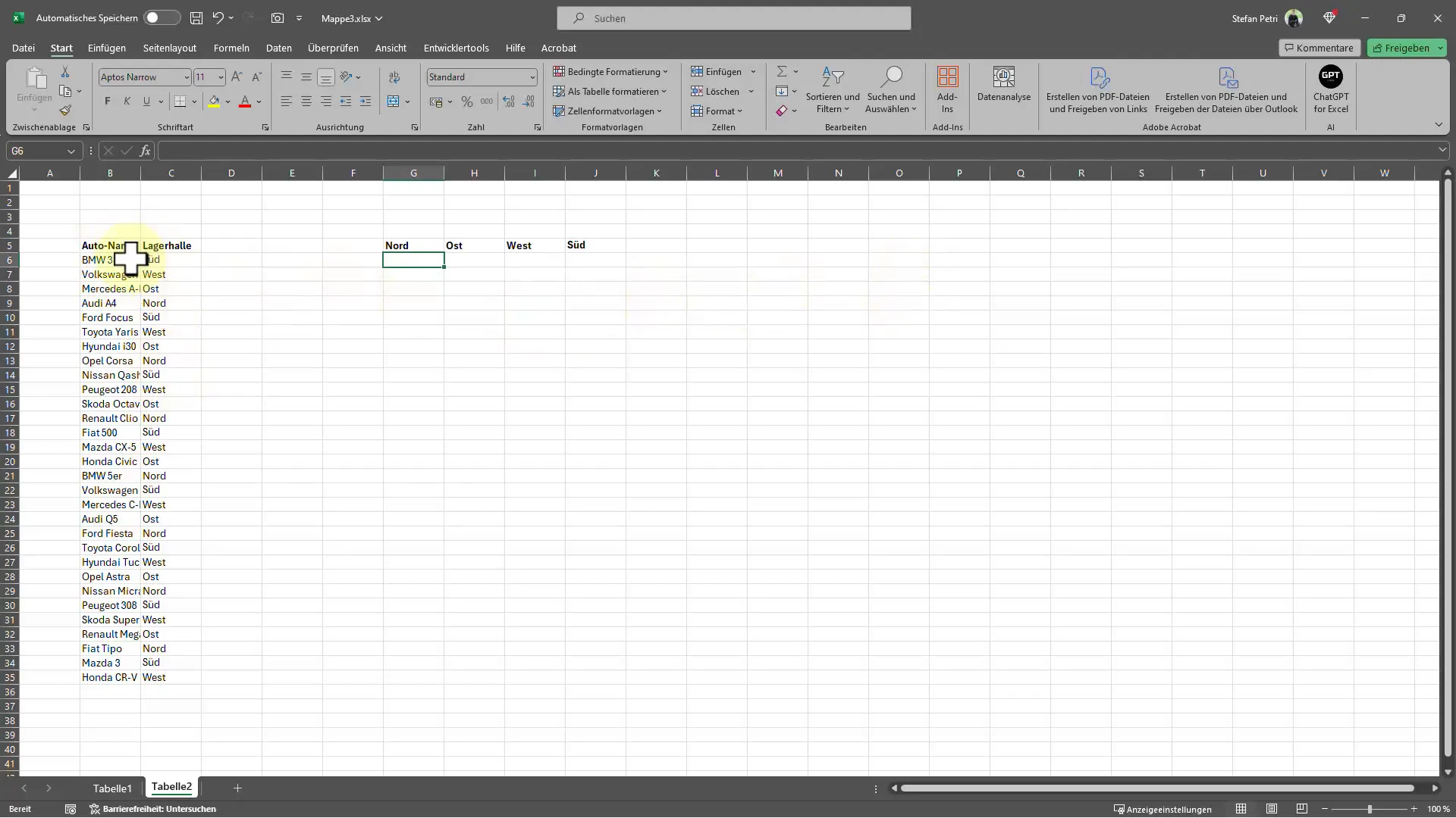
With the "Filter" formula, you can select the column with the car names. To ensure that the formulas do not get mixed up when making later adjustments to the table, you use the F4 key. This function ensures that the references are not readjusted when moving or copying the formula. Note: Each Excel language version may have different formula designations.

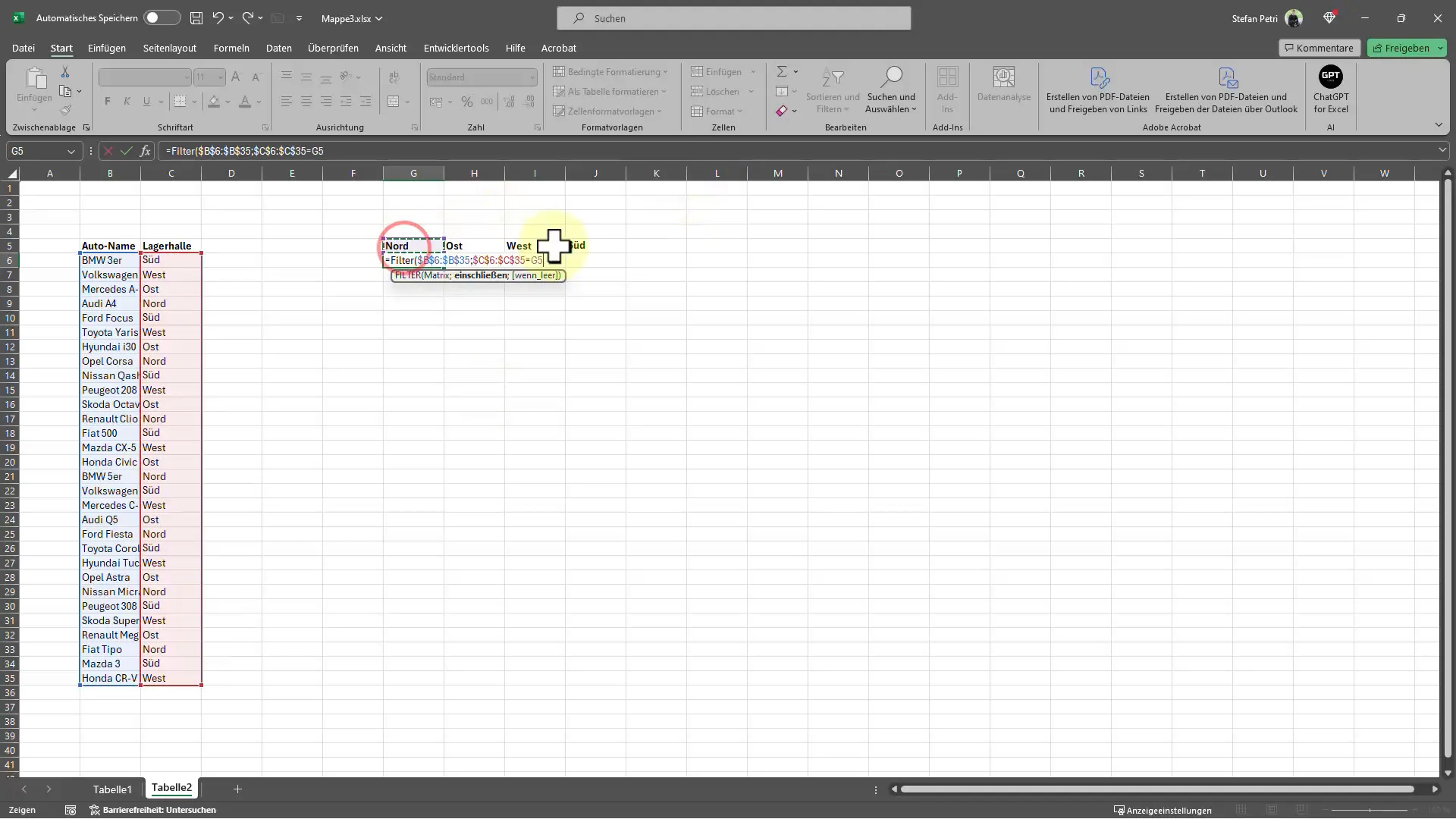
After selecting the entire column with the car names, press the F4 key again. Next, you insert a semicolon and select the second column that should also be filtered. Don't forget to press F4 here as well to fix the reference. In the window that opens, enter the column name to be filtered next.

Displaying the Filtered Data

Once you have successfully set up the filter formula, you can display the data in the new table. This table will now automatically show the corresponding car types filtered by location. This gives you a quick and direct overview of where each car is located.

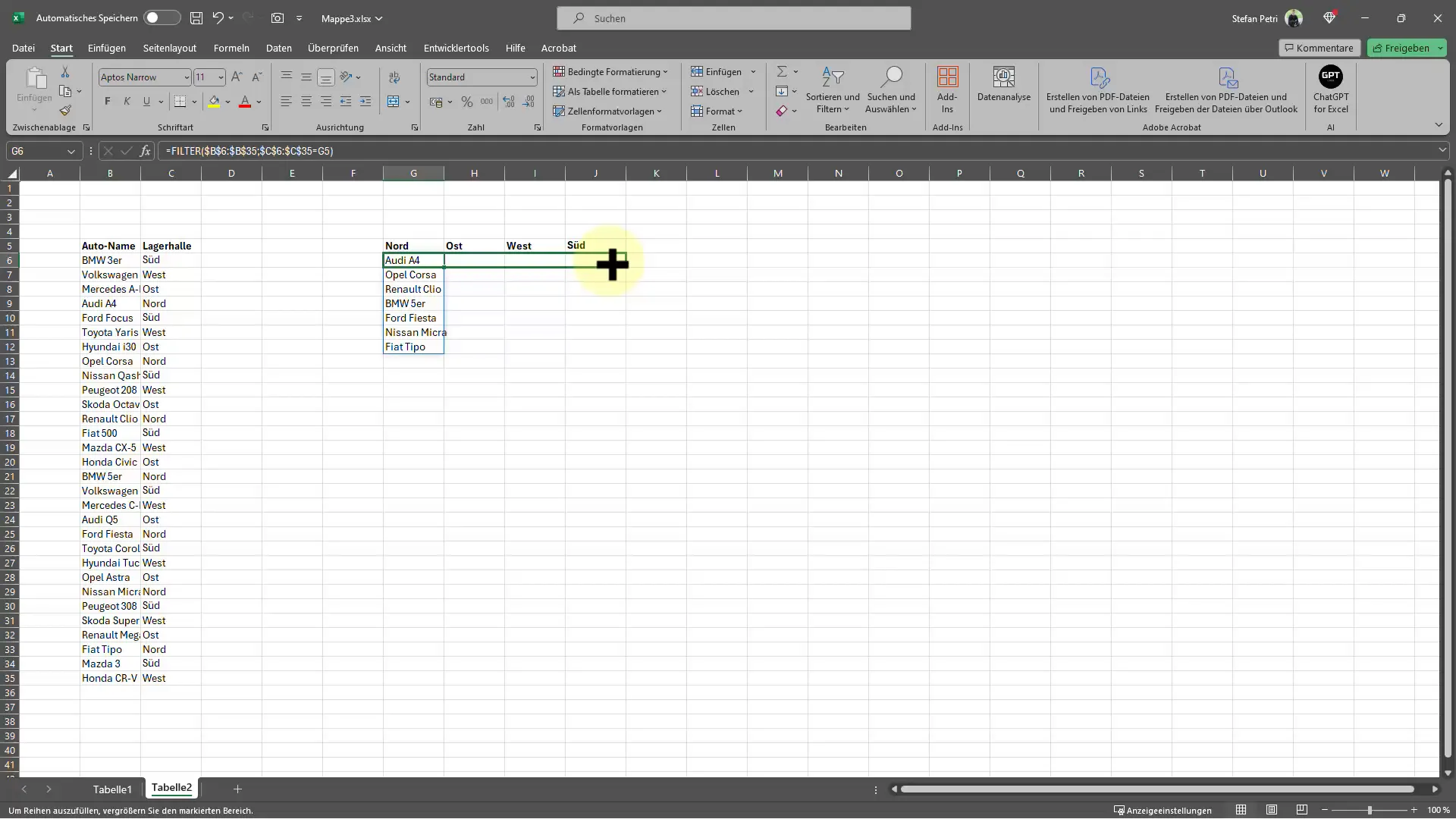
One of the major advantages of this method is its flexibility. You can change the filtering criteria at any time to display only the data that interests you. For example, if you only want to see the cars located in the North, you can easily adjust that.

If you want to create a table instead to utilize the filtering function, follow these steps: Click on the "Create as Table" button. This will optimize your data view, and you can filter directly from the table.

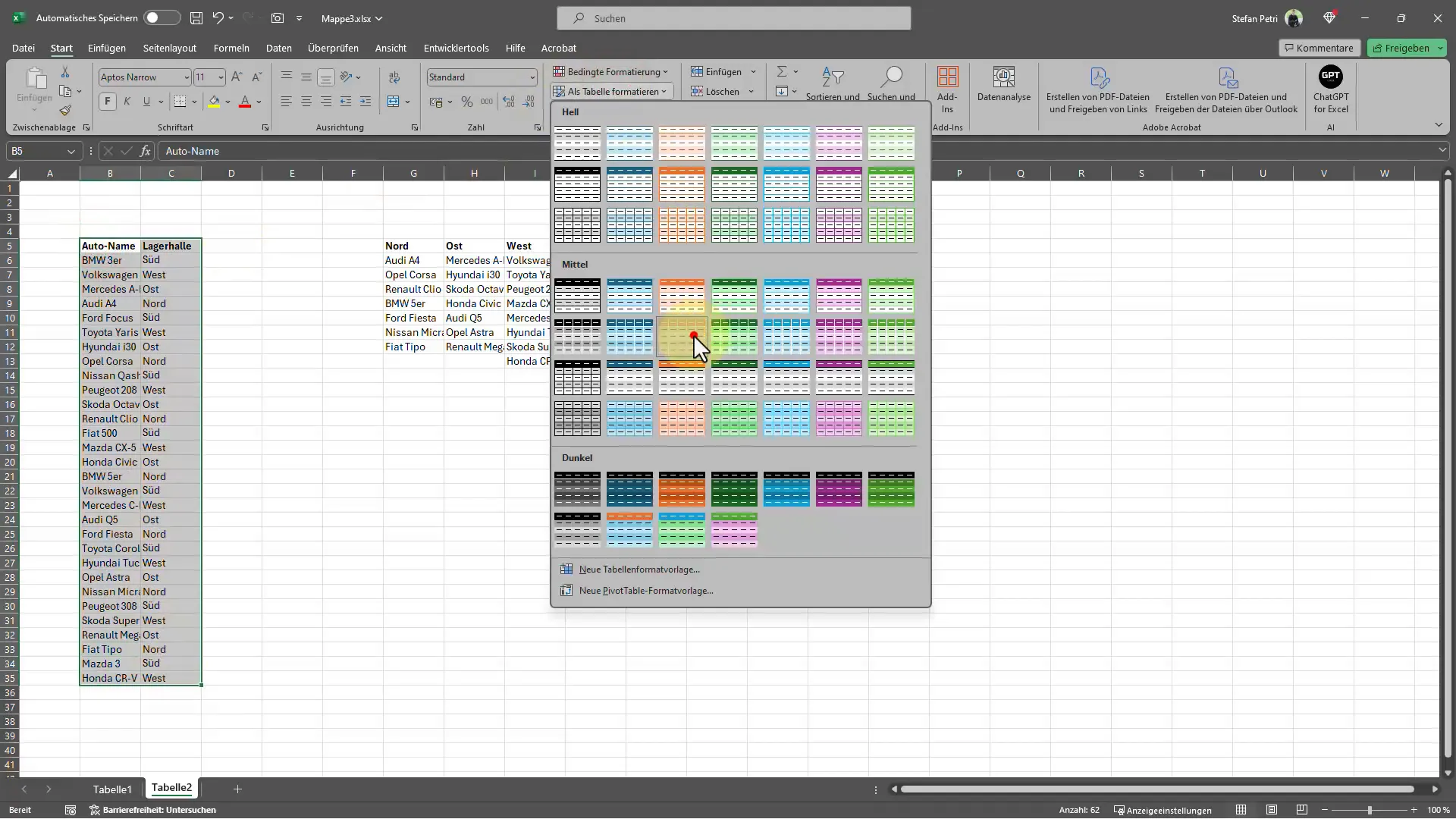
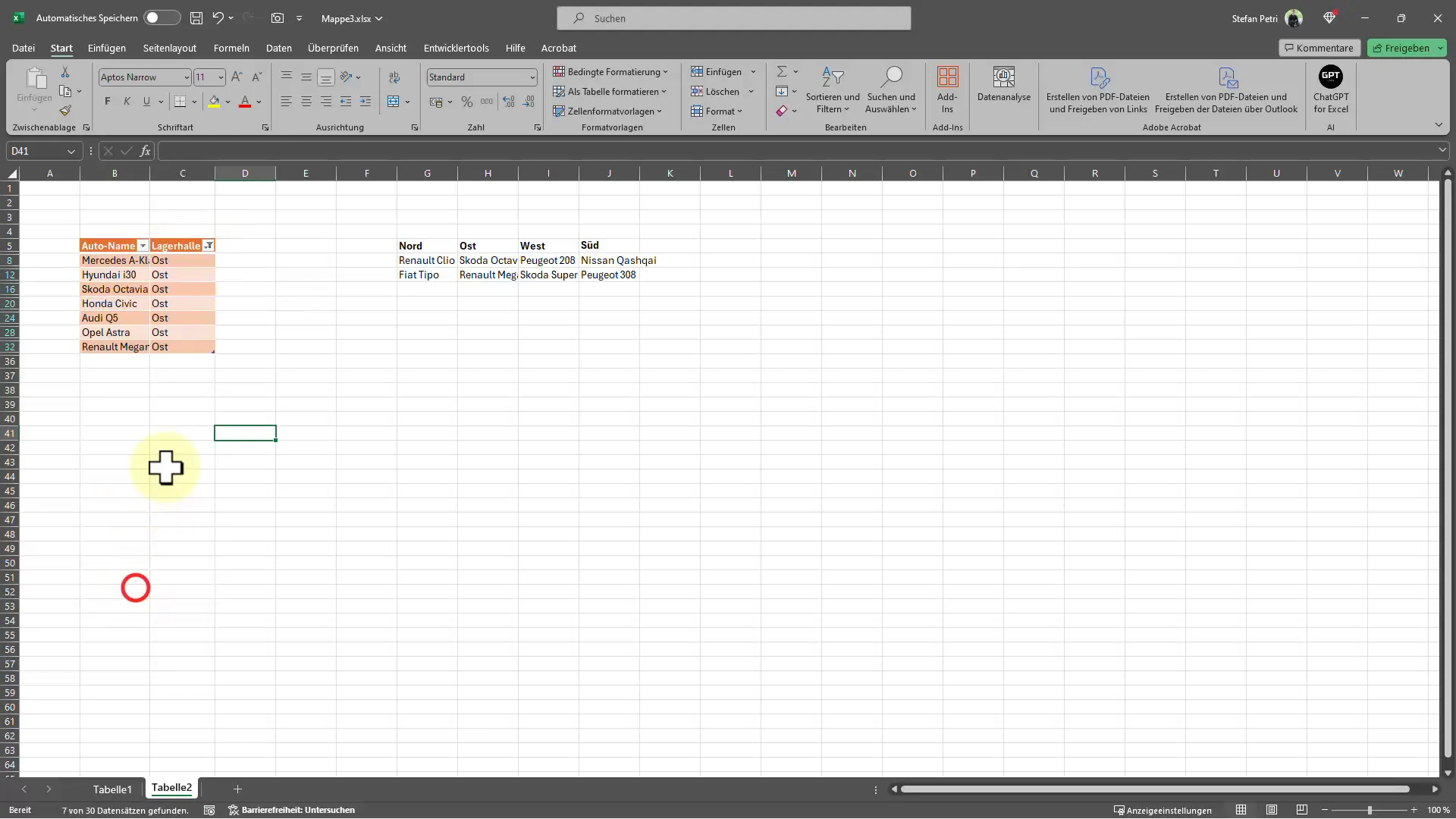
Then select the relevant columns and filter the desired warehouse, for example, only the cars in the North, East, West, or South. Note that using the table could affect the function of your previous filter formula.

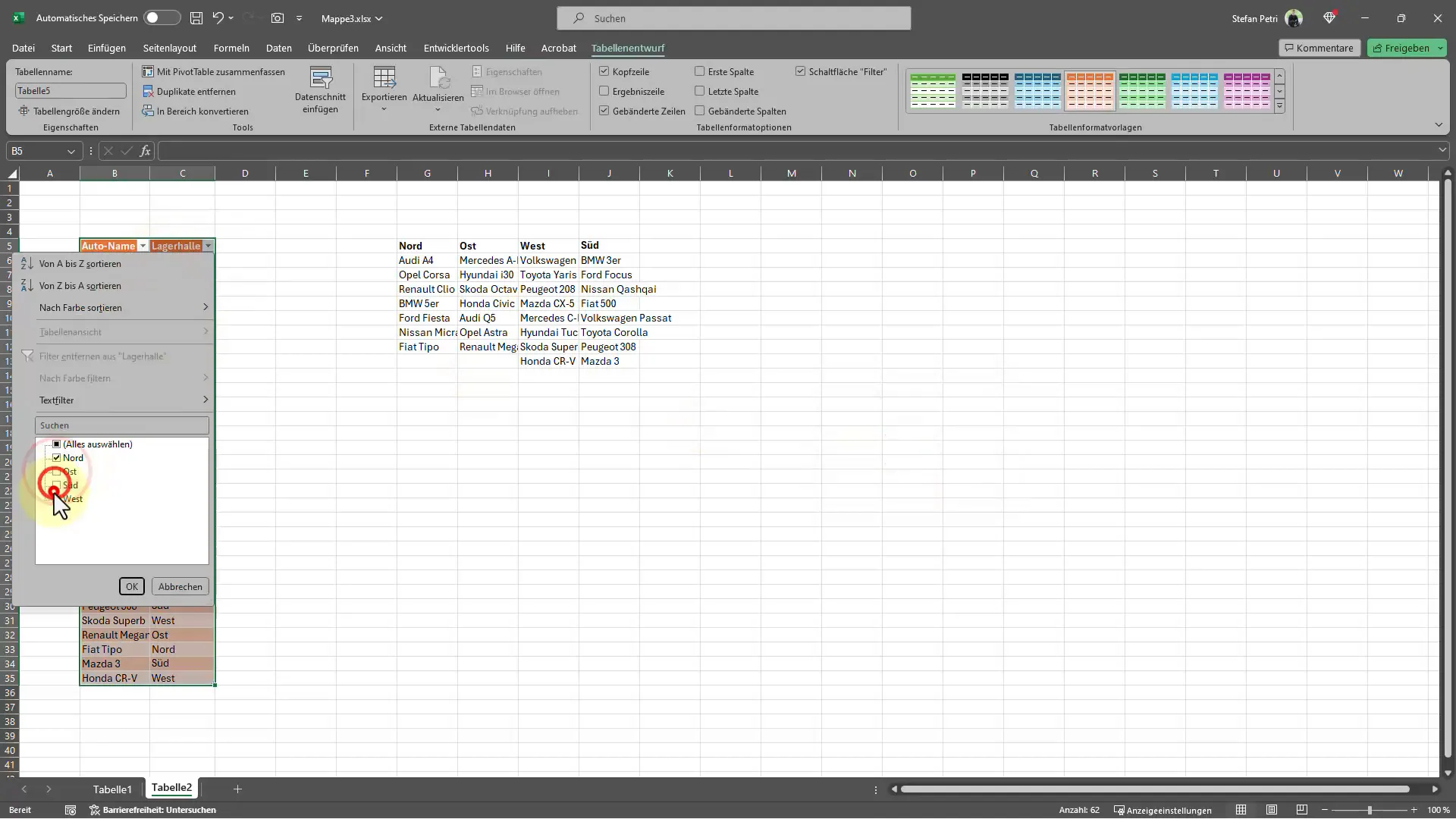
However, it is an equally useful method to improve the clarity of your data. In my case, I have only displayed the cars from the East warehouse.

Conclusion and Tips for Filtering Data in Excel

In conclusion, using the filtering function in Excel is an excellent way to extract specific information from large amounts of data. By combining filter formulas and tabular views, you gain control over your data. Remember to use the F4 key regularly to ensure that your data references remain correct, especially when making changes.