Effective filtering of data in Excel – Here's how you proceed

Filtering data in Excel is an essential skill that helps you quickly find and display relevant information. In this tutorial, I will show you how you can filter data even better than you are used to. Whether you are looking for specific brands in a vehicle database or just want an overview of large data sets – with the right filters, you will succeed. Let's dive right into the steps!

Key Insights

• Formatting data as a table automatically activates filter options.
• Using slicers simplifies filtering.
• You can apply filters to both columns and rows.

Step-by-Step Guide

First and foremost, it is important to organize the data you want to filter in a table. You can simply select your data and format it as a table, which I will explain to you in more detail now.

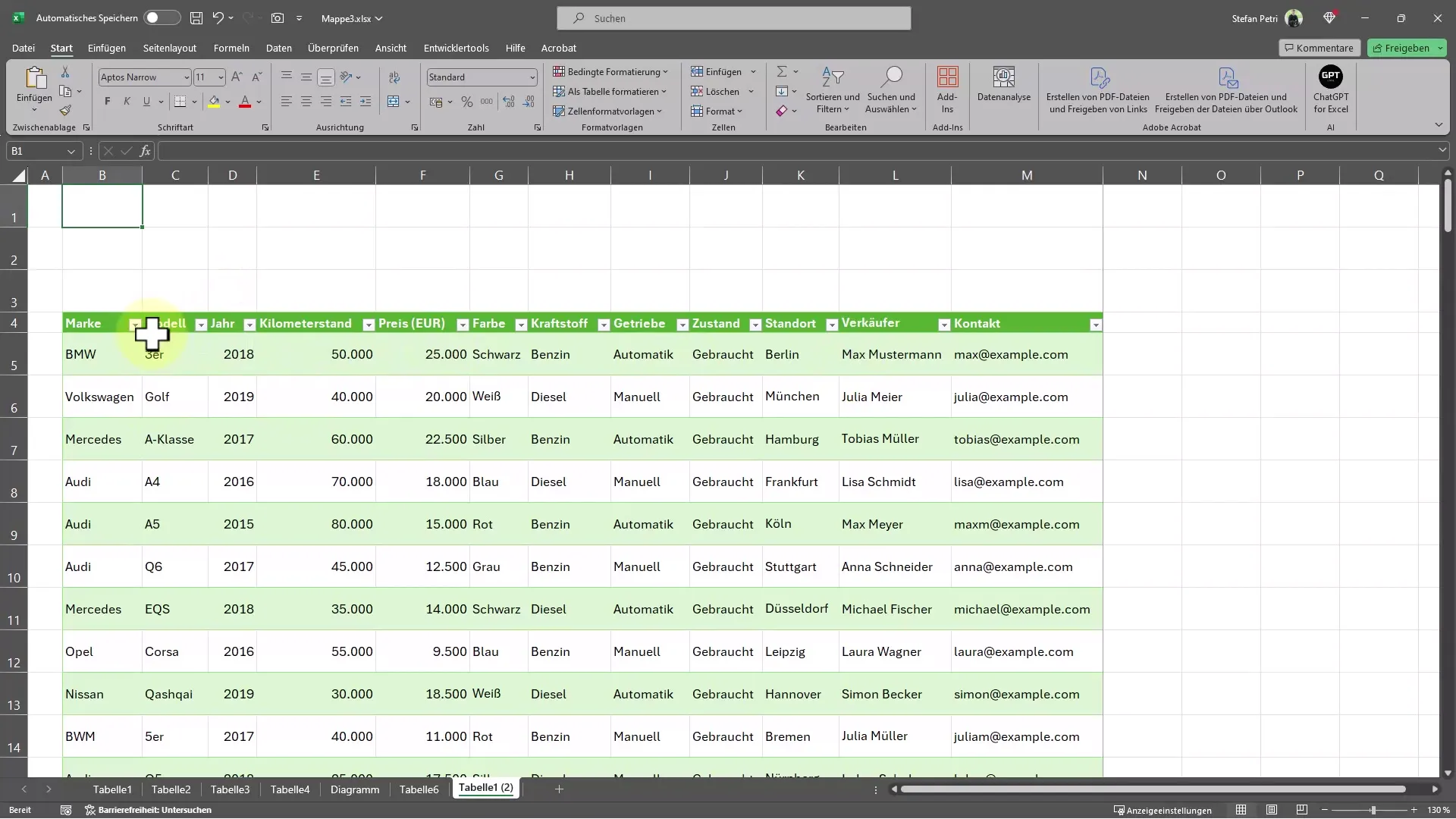
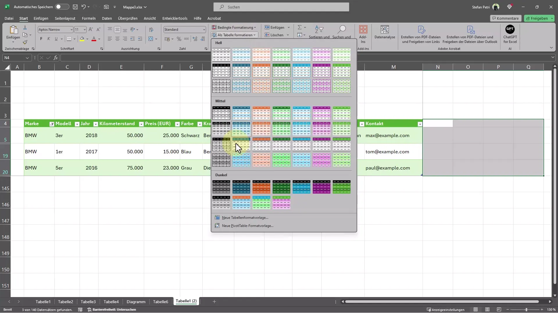
Start by selecting the entire table. You can easily do this by using the keyboard shortcut Ctrl + Shift + ↓ and the right arrow key to make sure you are selecting all the data. Now you can click on "Format as Table" under Home and choose one of the numerous templates. Or simply use Ctrl + T.

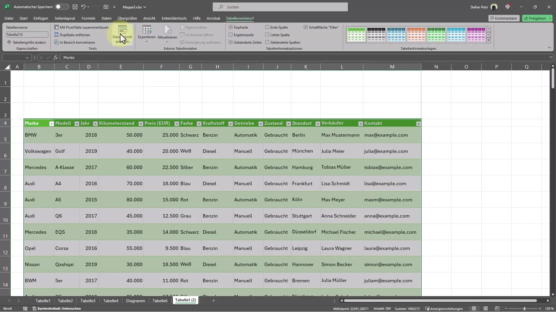
Once you have selected the data, go to the Table Design tab and click on Insert Slicer. This function allows you to choose the most important criteria for filtering.

Another important element is brand selection. If, for example, you only want to display BMW vehicles, select "Brand" as your filter option. All available brands will be listed, and you can easily apply the filter.

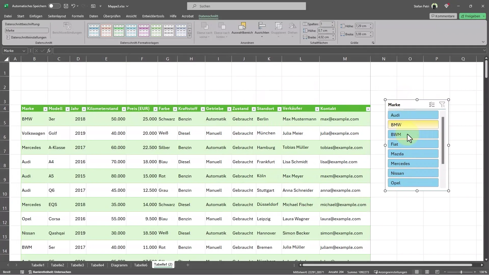
If you spot a typo, like "BMY" instead of "BMW", you can correct it right away while applying the filters. It's a great way to ensure everything is correct as you go through the data.

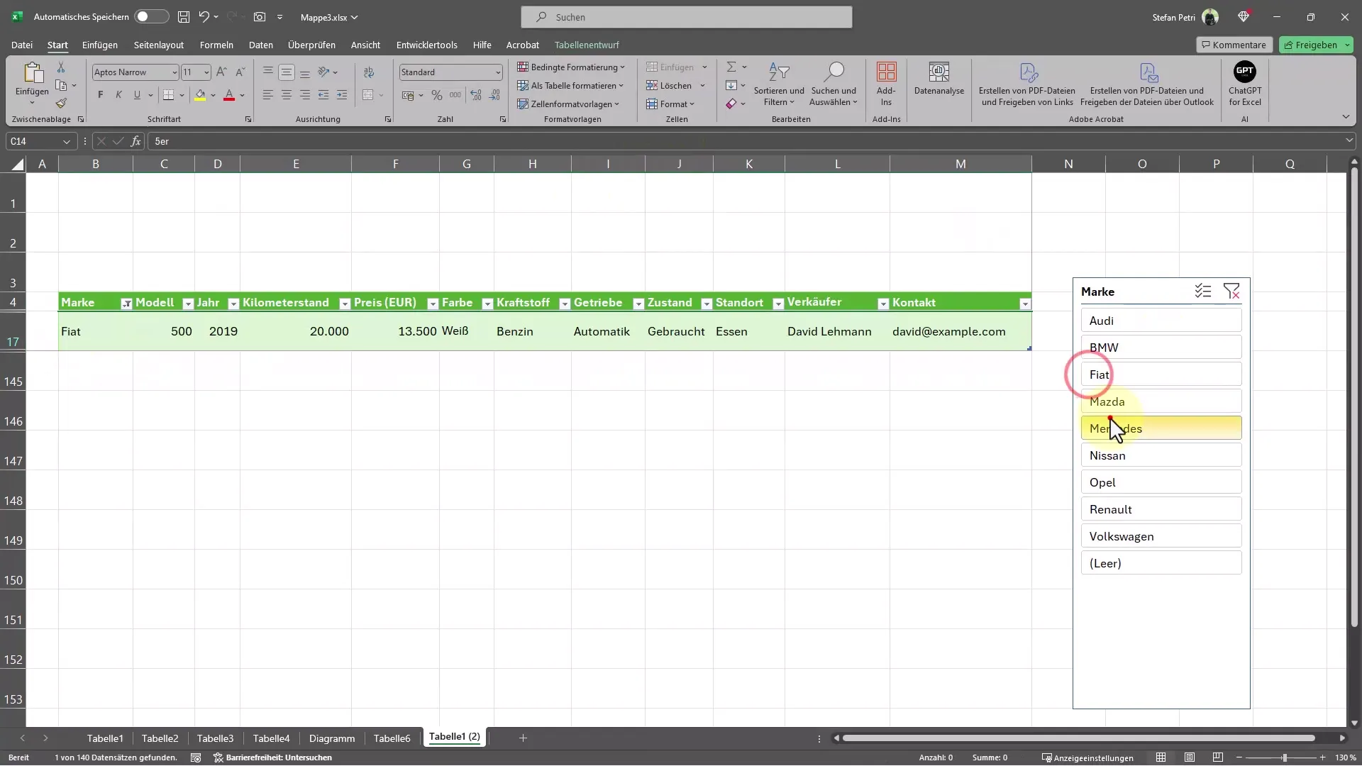
In addition to filtering columns, you also have the option to filter data by rows. To do this, go back to the Slicer and select the columns you want to filter. This is especially helpful when you have many different categories you want to view simultaneously.

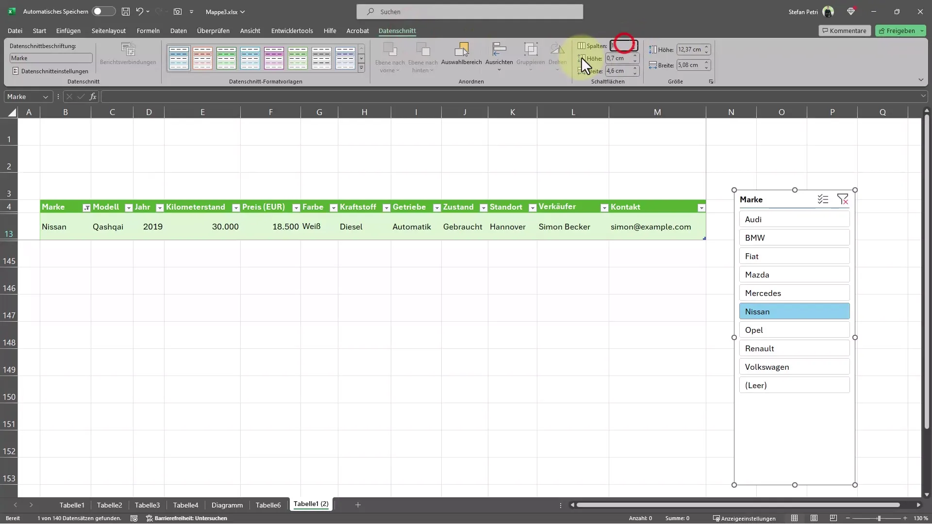
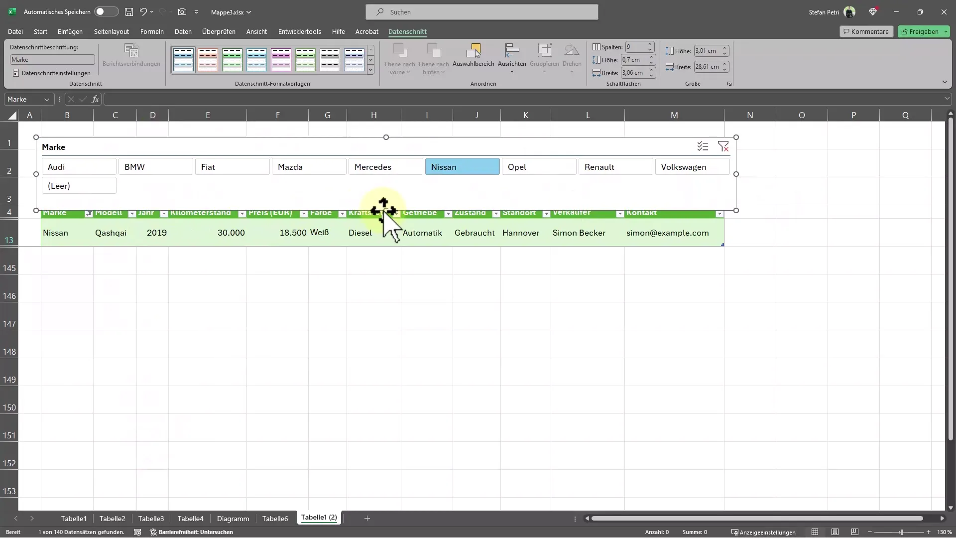
Then, drag the filter field to the desired size. This ensures that all information fits and is clearly visible.

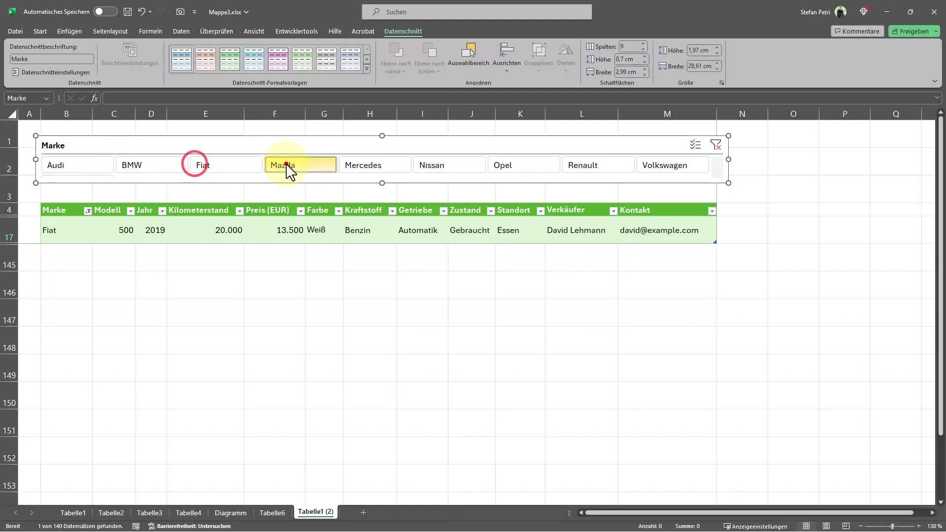
Now you have the ability to efficiently filter the desired information and quickly see which vehicles are included in your database.

Summary

By filtering data correctly, you get the exact information you need without being distracted by irrelevant data. By following the steps above, you can analyze and present your data much more effectively.