Quickly find data using the VLOOKUP function in Excel

When working with large tables in Excel, it can be very tedious to find the necessary information. The VLOOKUP function (Vertical Lookup) is a powerful tool that helps you quickly and efficiently search for and display data. In this guide, I will show you concrete steps on how to easily use the VLOOKUP function in your Excel file, for example, to find product information based on a number.

Main Insights

• The VLOOKUP function enables a quick and uncomplicated search in large datasets.
• With VLOOKUP, you can not only search for unique entries, but also display multiple values by adapting the function accordingly.
• VLOOKUP supports the combination of multiple functions to obtain tailored results.

Step-by-Step Guide

First, make sure your data is in a structured table. It is important that the first column contains the search criteria (for example, product numbers).

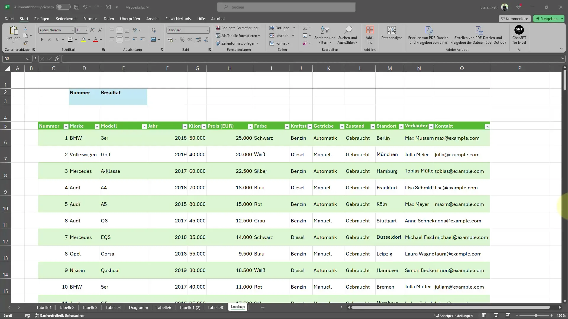
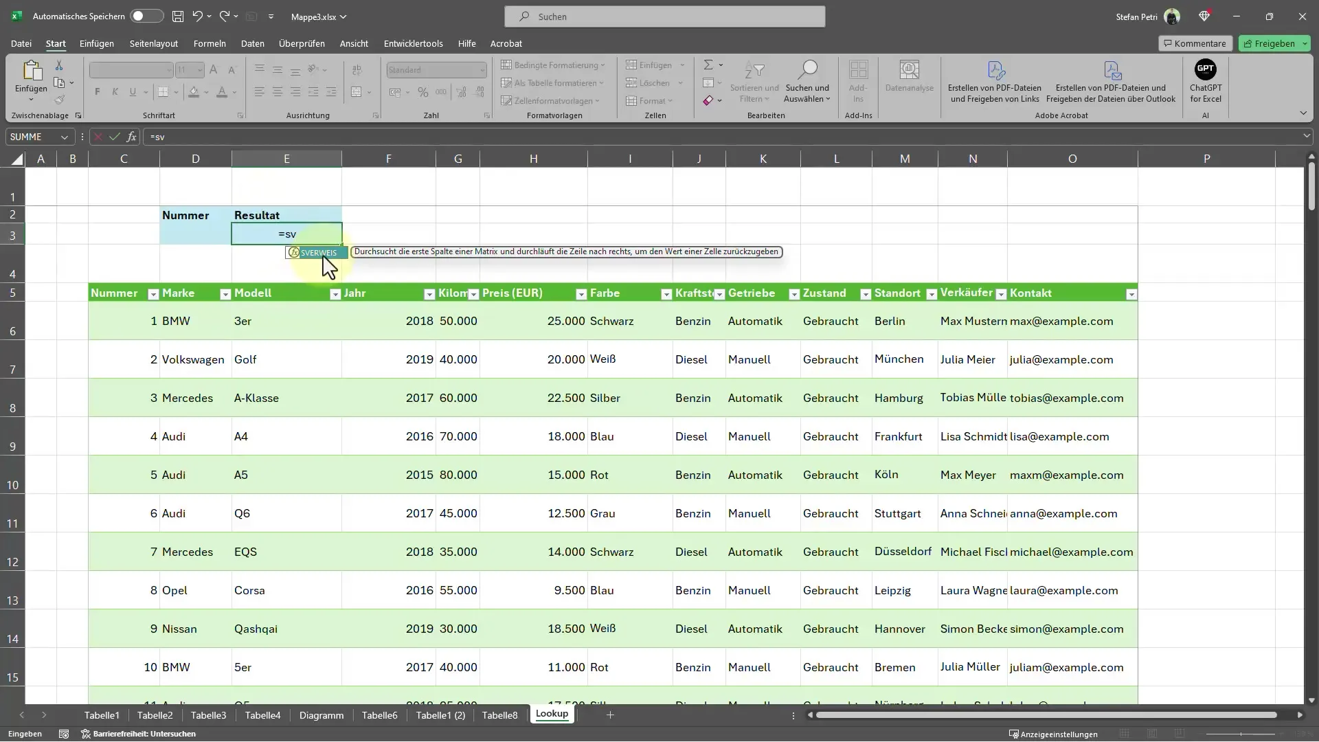
At the beginning, I want to show you the most basic application of the VLOOKUP function. To use the function, simply go to the cell where the result should be displayed and enter the following formula:

=VLOOKUP(...)

Here you fill in the three main arguments of the function. In the first step, you specify the search criteria. This means that you must enter the number of the product you are looking for here.

Next, add a semicolon to the formula and select the range that contains the data you want to search. Typically, this range includes all relevant columns in your table.

Now add another semicolon and specify the column index that indicates from which column the result should be displayed. For example, if you want to know the brand of the product, you add the number of the corresponding column.

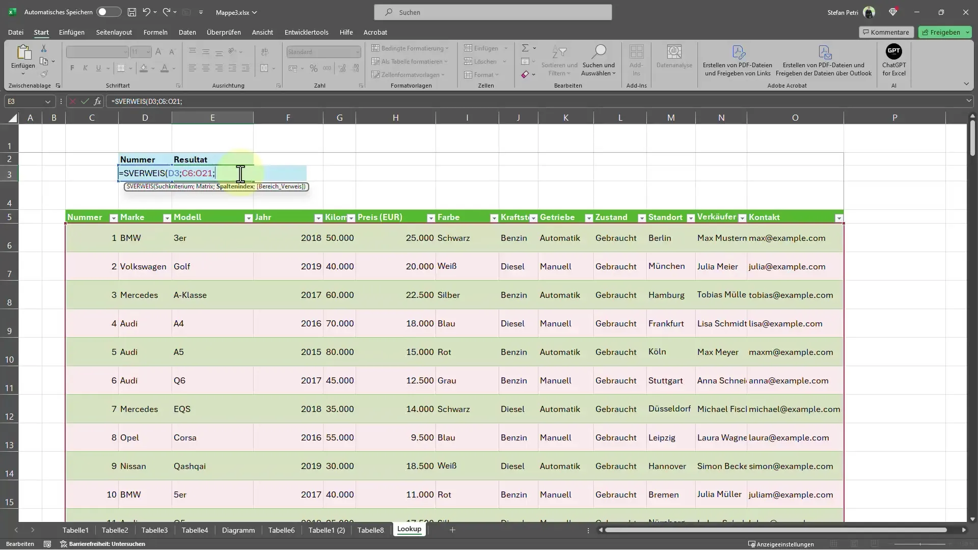
The next argument is the exact match. By default, it is recommended to use the "FALSE" value here to ensure that only exact matches are displayed. To complete the formula, close it with a parenthesis.

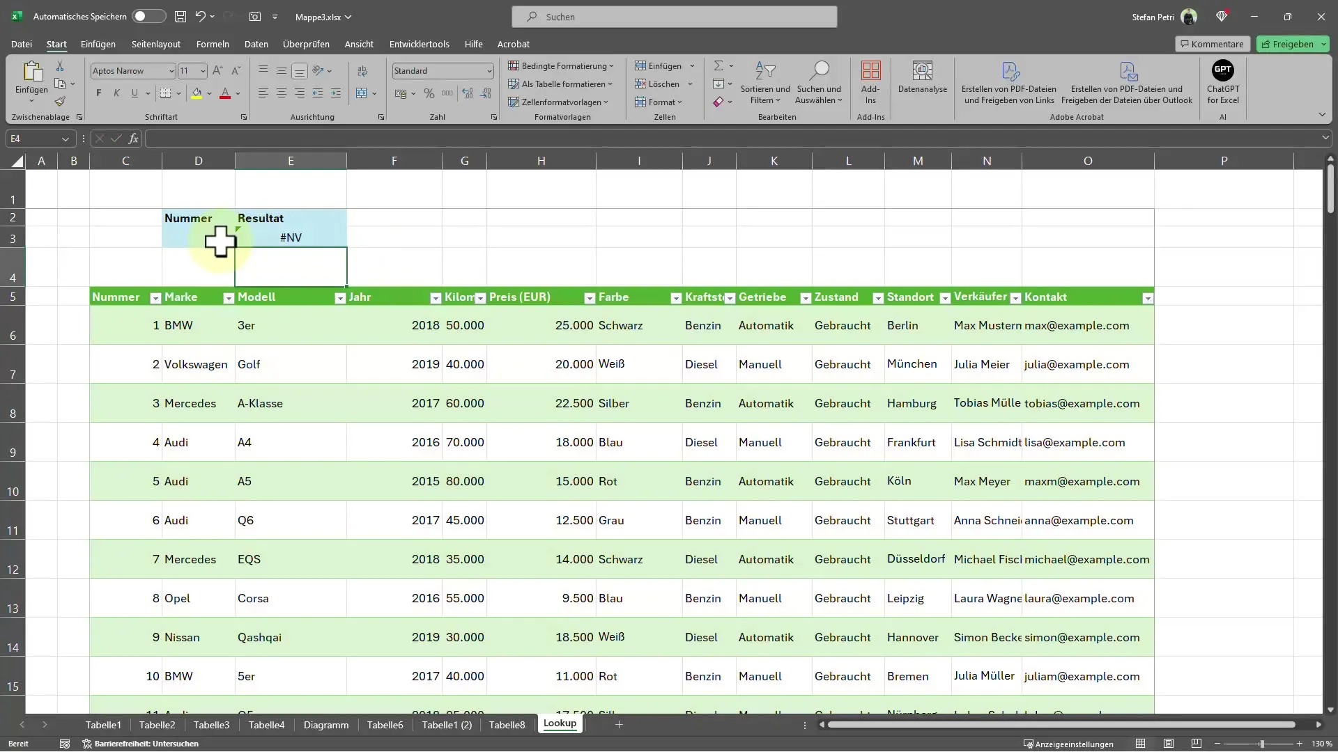
Now you can get the result. For example, if you enter the number 2, "Volkswagen" will be displayed, and for number 4 you will see "Audi".

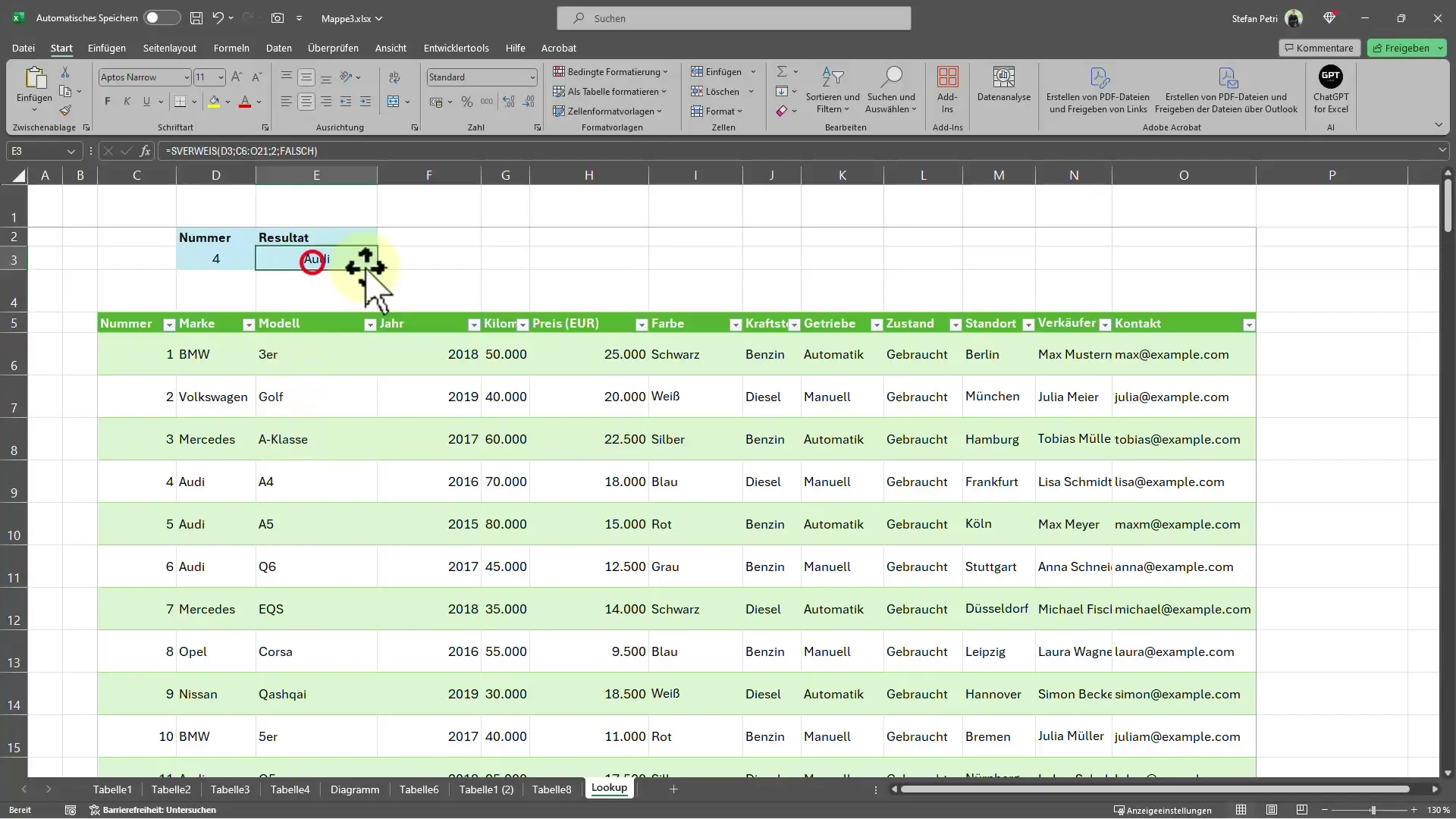
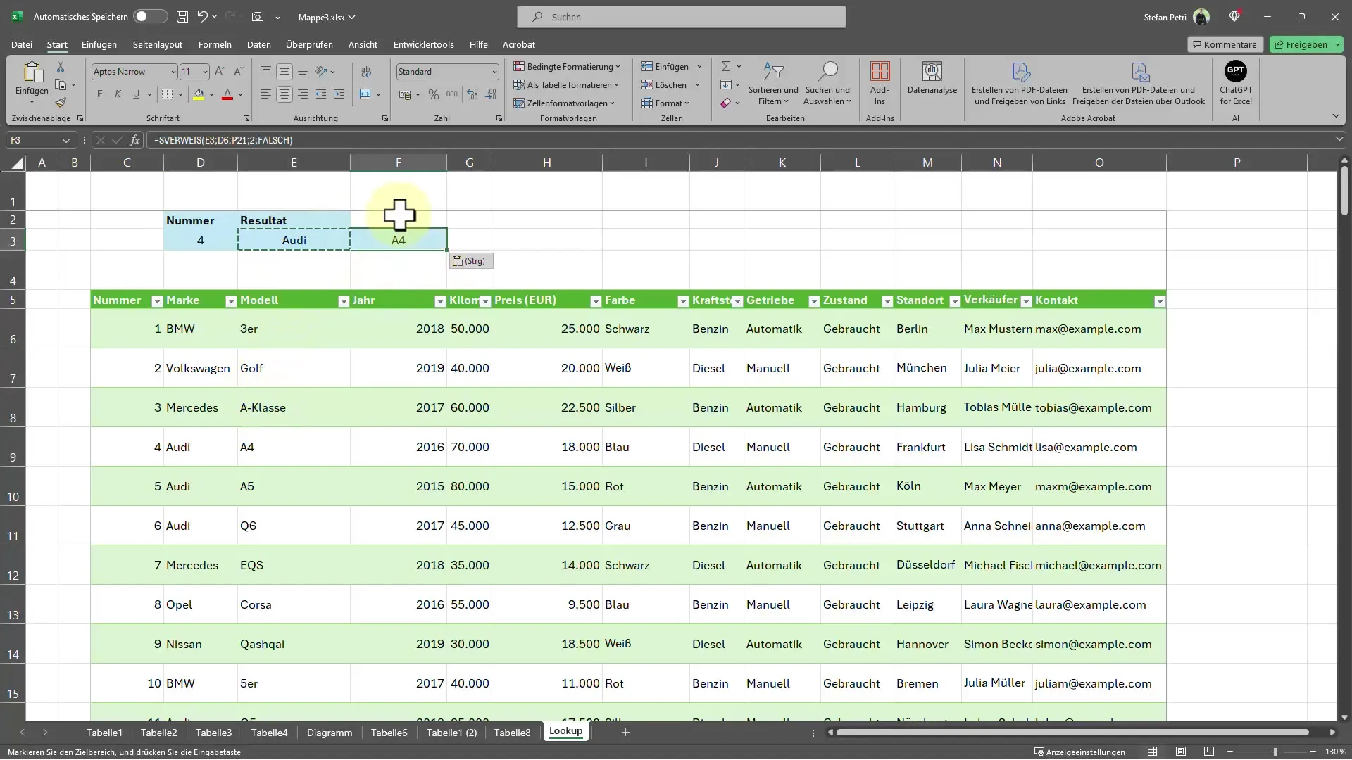
But you might also want to see more detailed information about the product, such as the model. In this case, you need to copy the formula by copying the current cell content with CTRL + C and then pasting it into another cell with CTRL + V.

If you want to combine the two pieces of information in one cell, you can do that as well. Remove the two previous formulas and add another function. Here, you use the ampersand (&) to separate the results. Add the VLOOKUP function again and remember to specify the corresponding column index.

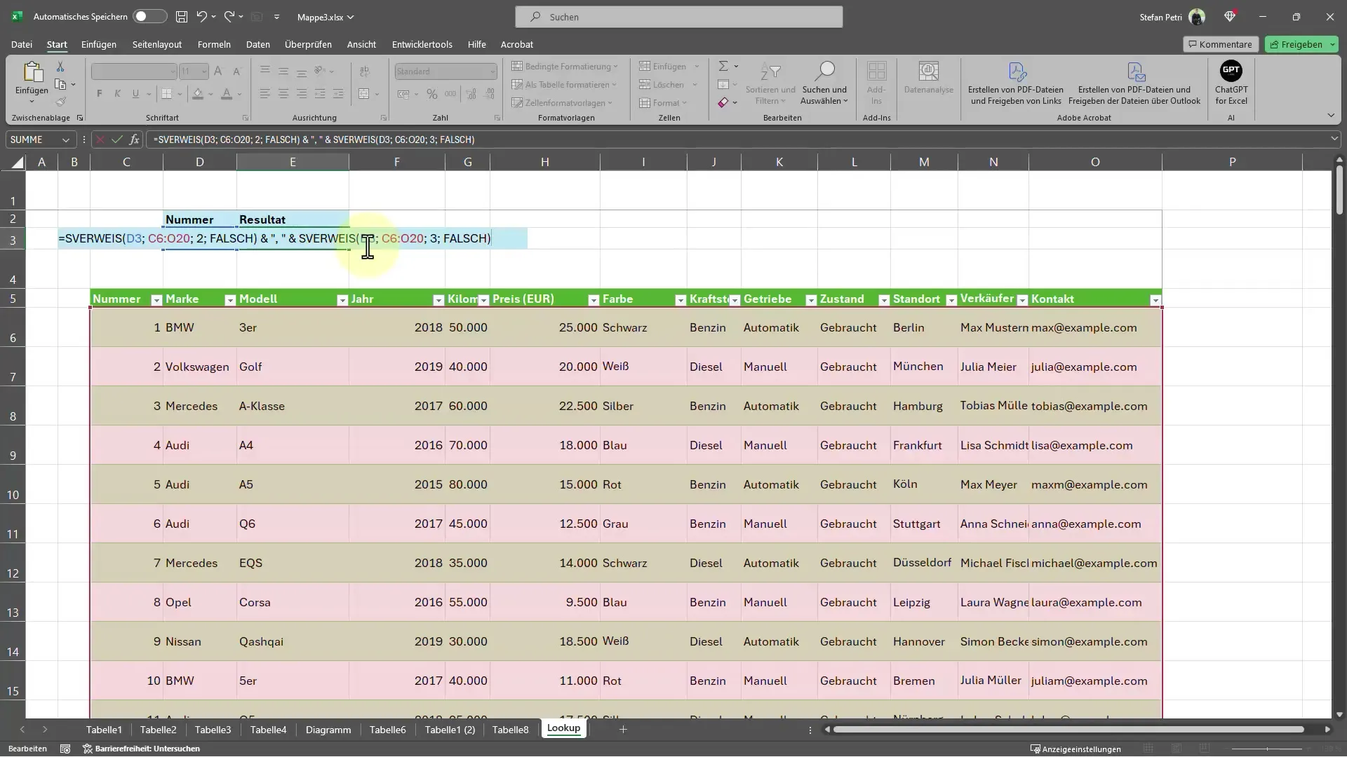
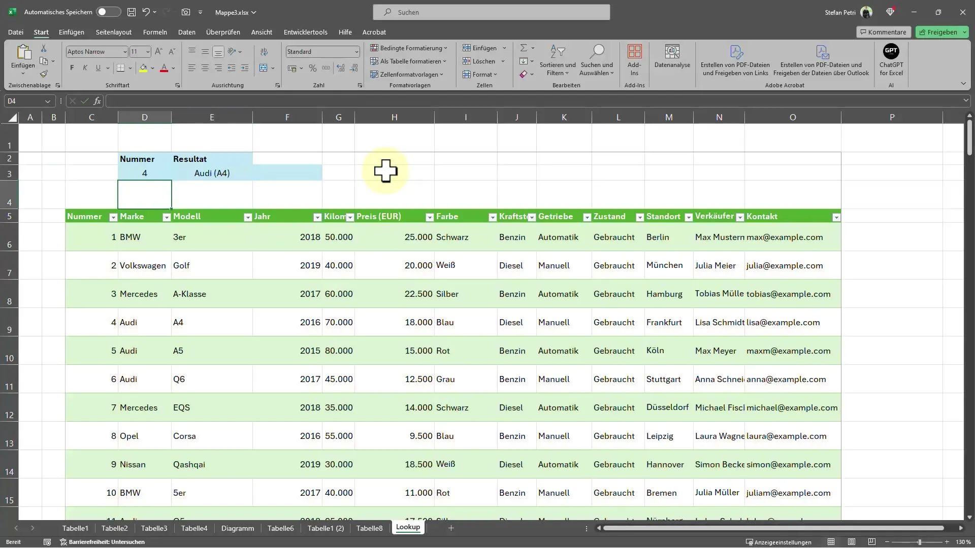
By finally pressing the Enter key, you will now get a cell that displays, for example, "Audi A4" or "Volkswagen Golf".

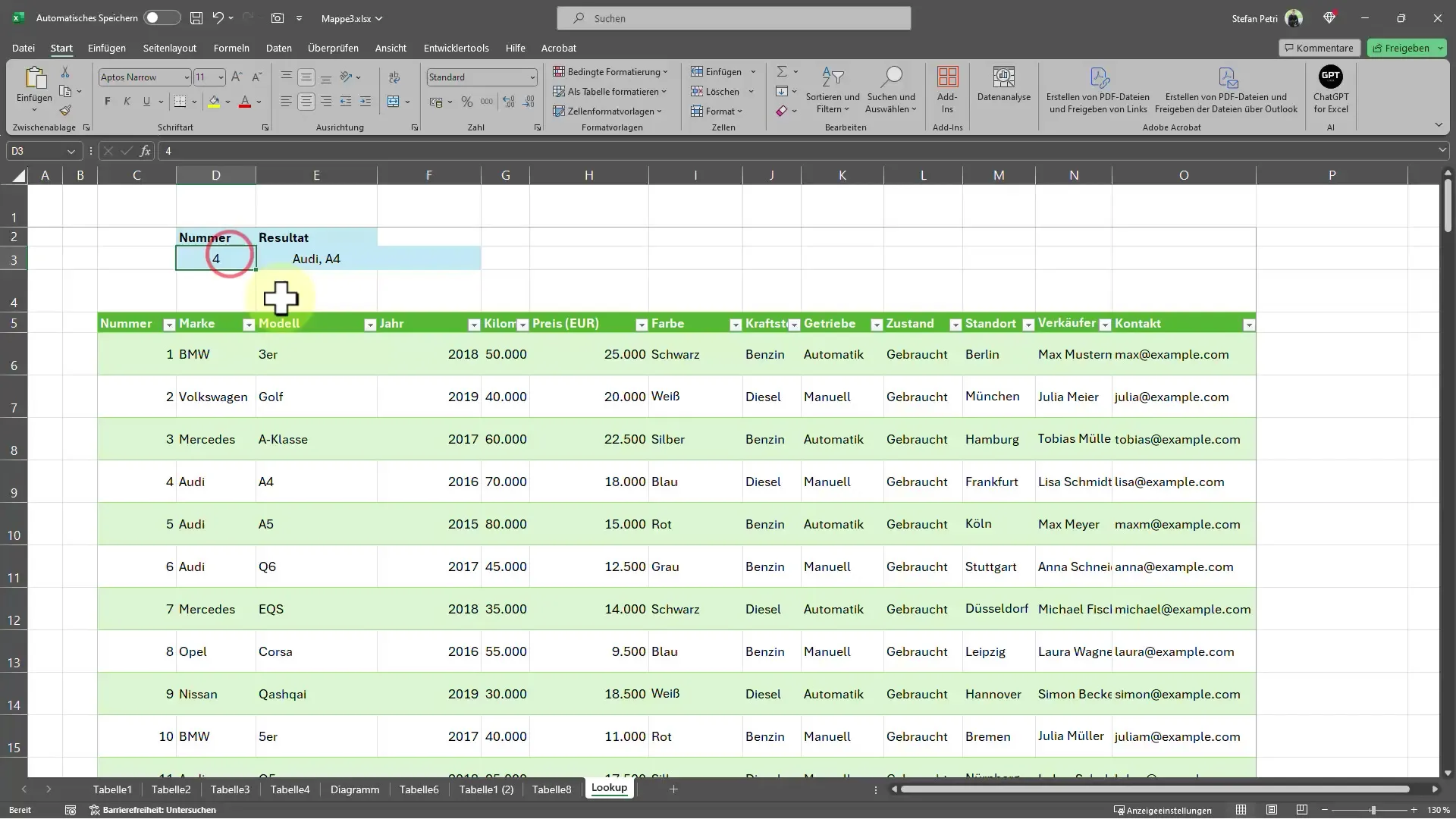
If you don't like the output format, you can also use different delimiters. Instead of a comma, you could use a space or another symbol.

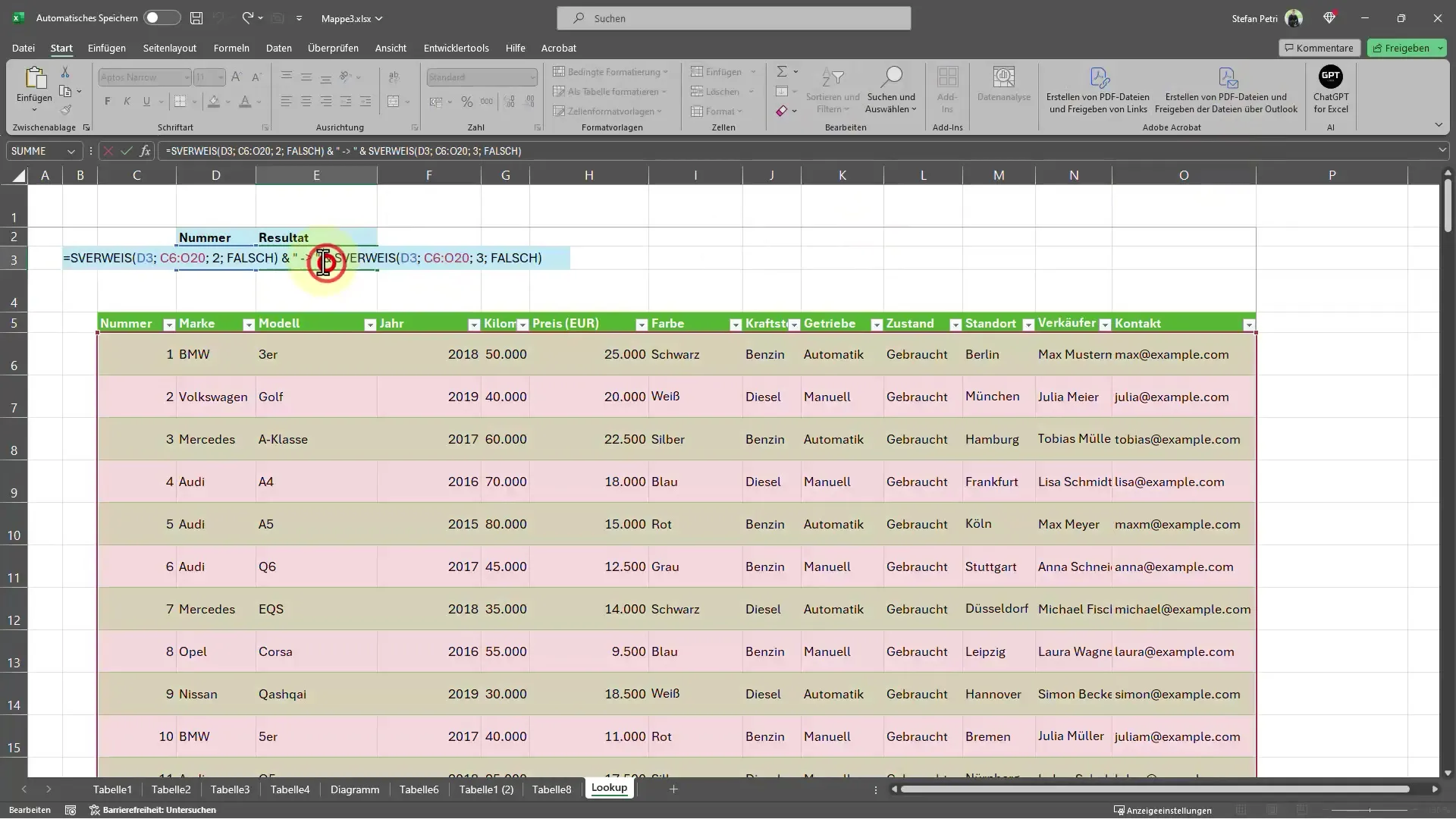
Now you have the information with the models in one cell, which significantly simplifies your work process.

Summary

In this tutorial, you have learned how to use the VLOOKUP function in Excel to quickly and effectively find product information based on a search number. By correctly applying this function, you can significantly improve your work with large amounts of data.