Displaying rating stars in Excel - Here's how!

As a user, you want to be able to quickly and easily see at a glance how good a product is. A very visual method to do this is by using rating stars. In this tutorial, you will learn how to display stars in a cell in Excel. Not only is this easy to implement, but it also enhances your tables and makes them more intuitive. Let's get started right away!

Main Insights

You can insert stars into an Excel cell by using a special formula based on the number of stars you want. You will also be able to use emojis to customize the appearance of the stars. Additionally, you have the option to change the colors of the stars to make the look of your rating more visually appealing.

Step-by-Step Guide

First, make sure you have Excel open and are ready to work with a new or existing table. Above all, you should have a column that is currently empty and will soon be filled with rating stars.

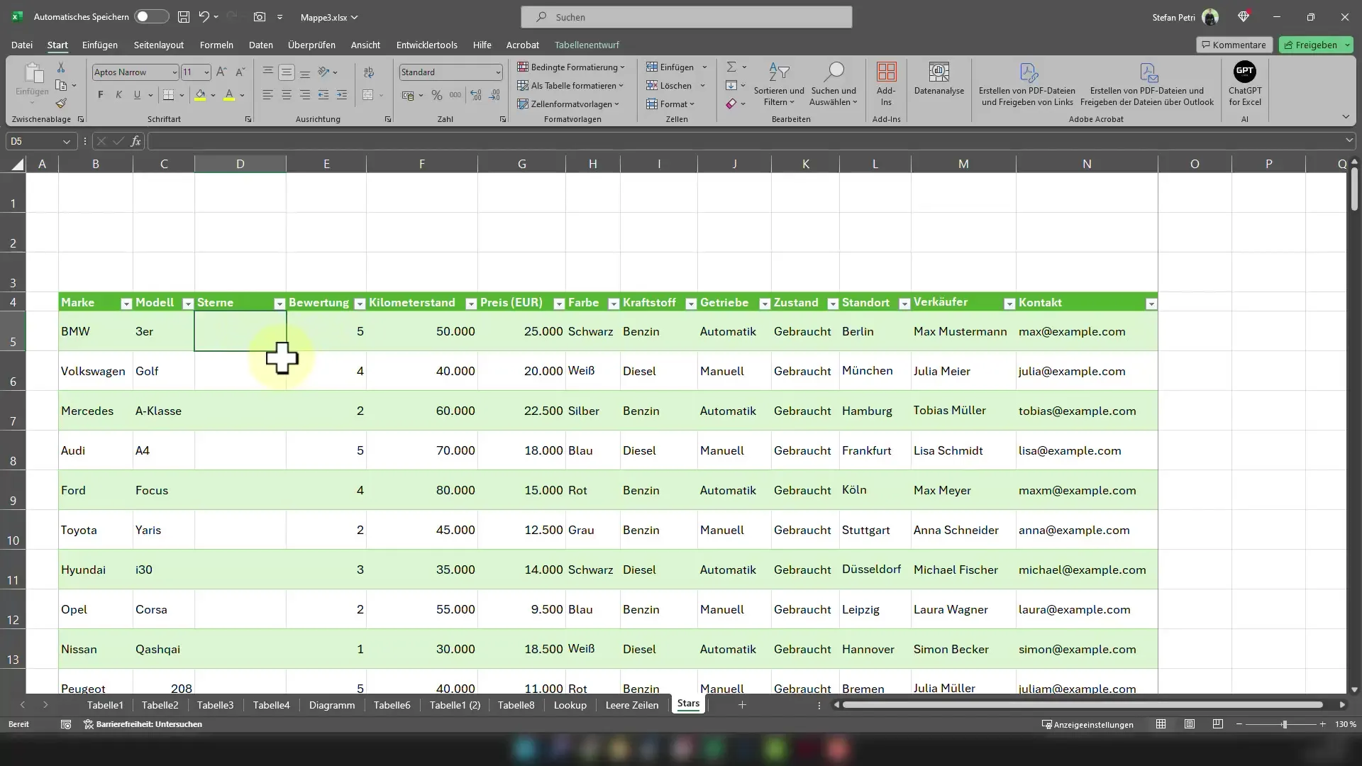
Step 1: Prepare the Formula

First, you need to enter the formula that allows you to repeat stars. The formula is called "REPT". To use it, type "=REPT(" and press the Windows key and the dot (•) symbol on your keyboard to insert the star symbol.

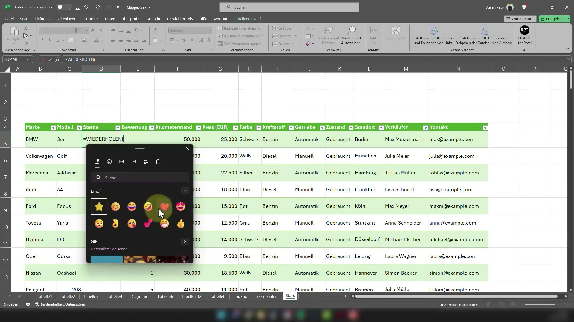
Step 2: Define the Text and Rating Basis

Make sure to use the semicolon after the star symbol and then add the cell reference from which the rating (e.g., the number of stars) should be derived.

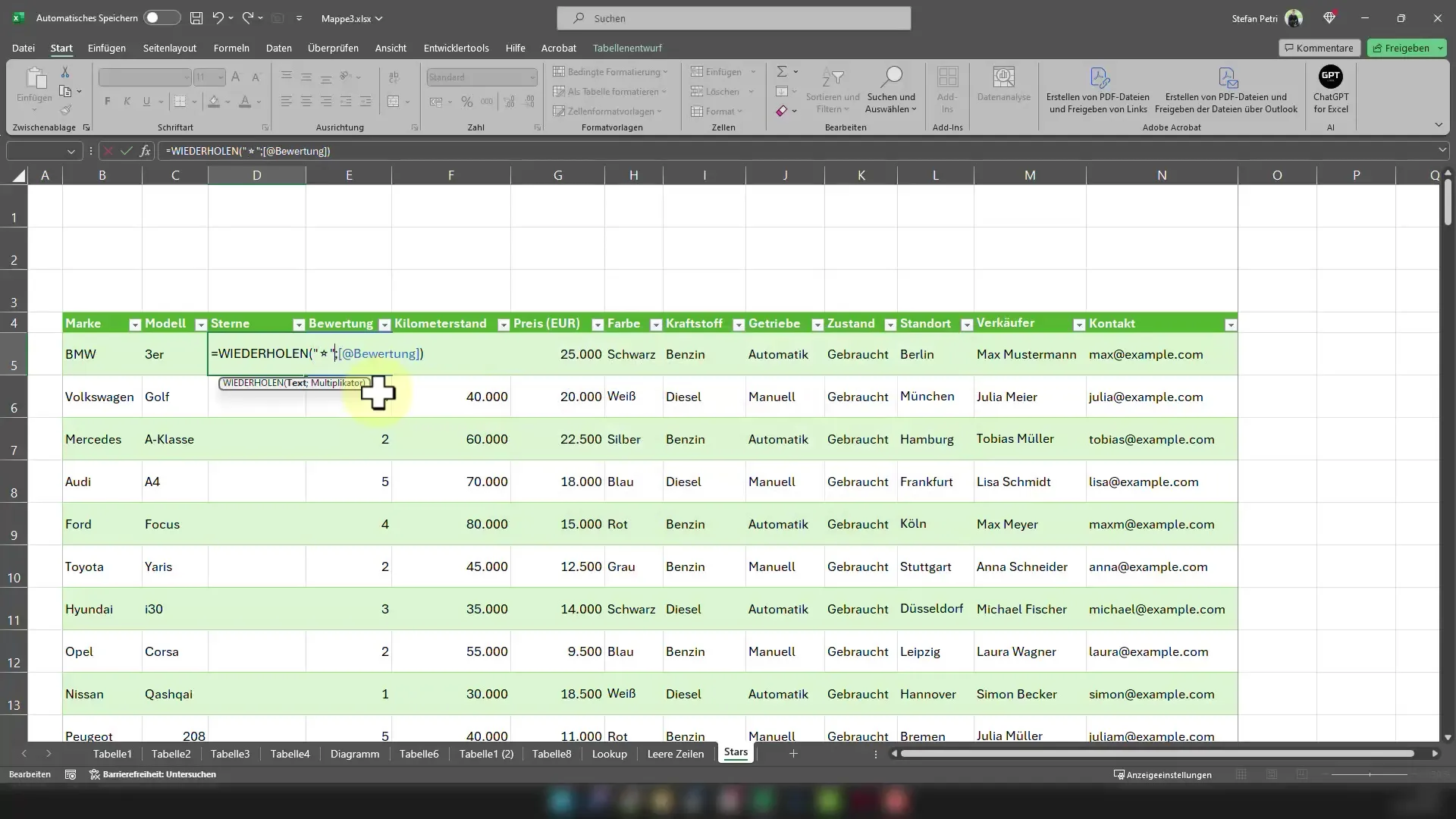
Step 3: Complete the Formula

To fully execute the formula, all the parameters must be contained within quotation marks. Add the cell reference and close the parenthesis. If you press "Enter" now, you should be able to see the corresponding stars in your cell. If you encounter issues, it often helps to check the quotation marks or parenthesis.

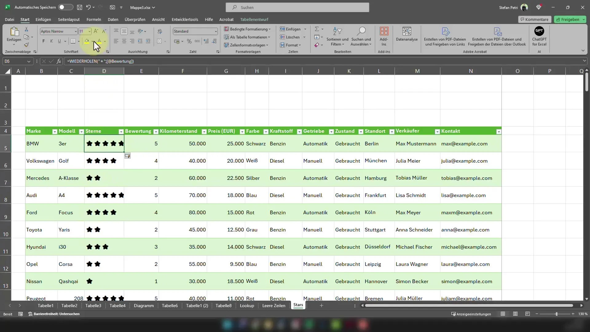
Step 4: Customize Star Colors

To visually enhance the stars, you can adjust their color. Select the cell and use the key combination "Ctrl + Shift + Down arrow" to change the color to yellow. This will bring the stars to life and make them clearly visible to your viewers.

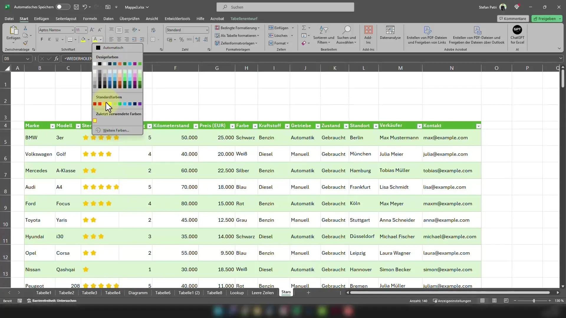
If yellow does not have the desired effect, try different colors. For example, you can also switch to a soft orange, which often better suits the overall aesthetic.

One of the cool features of your formula is its flexibility. Simply change the rating in the referenced cell and watch as the number of stars changes in real-time. For example, if you need a rating of six stars, you can easily adjust the number and it will be displayed accordingly.

Summary

Inserting rating stars in Excel is a simple yet effective way to visually present your data in a compelling and intuitive manner. By combining simple formulas and using emojis, you can add color and life to your worksheet. This creates a clear, immediate perception of product reviews or similar data that benefits users.