Excel tips: Quickly modernize formatting of table

In today's tutorial, I will show you how to quickly and effectively modernize formatting in Excel tables. Often, manual adjustments to the table width and height take a lot of time, even though there are much faster ways to improve the appearance of your tables. I will show you various tips and tricks to help you make your tables visually appealing without losing much time. Let's get started!

Main Insights:

• You can efficiently format the table with simple keyboard shortcuts and mouse clicks.
• Automatic adjustment of row and column widths allows for better readability.
• With a few clicks, you can modernize the design of your table and greatly improve readability.

Step 1: Selecting the Table

To start formatting, you need to first select the entire table. In Excel, this is quite simple. You can directly click on the table or use the "Ctrl + T" keyboard shortcut to quickly select the entire table.

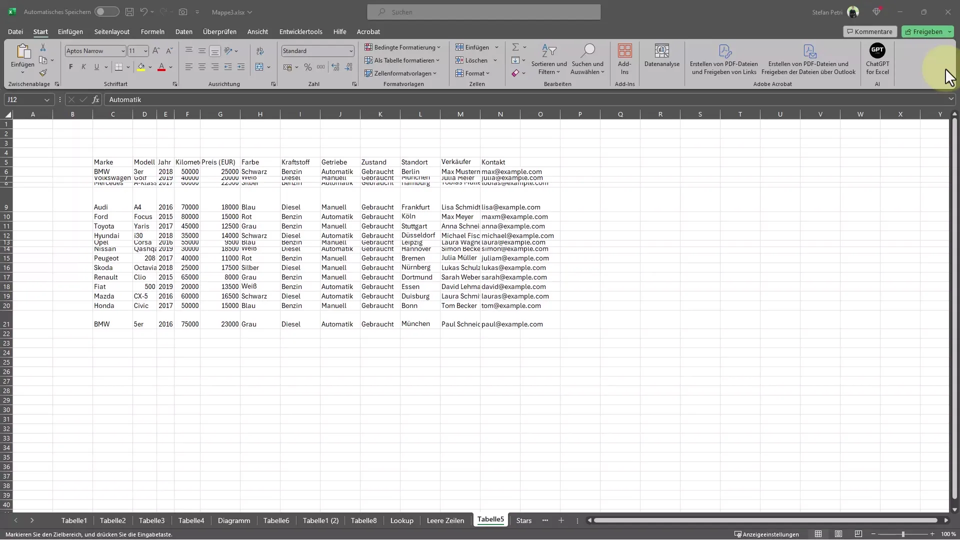
Step 2: Defining the Table Header

Once the table is selected, you can set a header. This improves readability and gives the table a structure. Simply click on the first row of your table and choose the function to format the header.

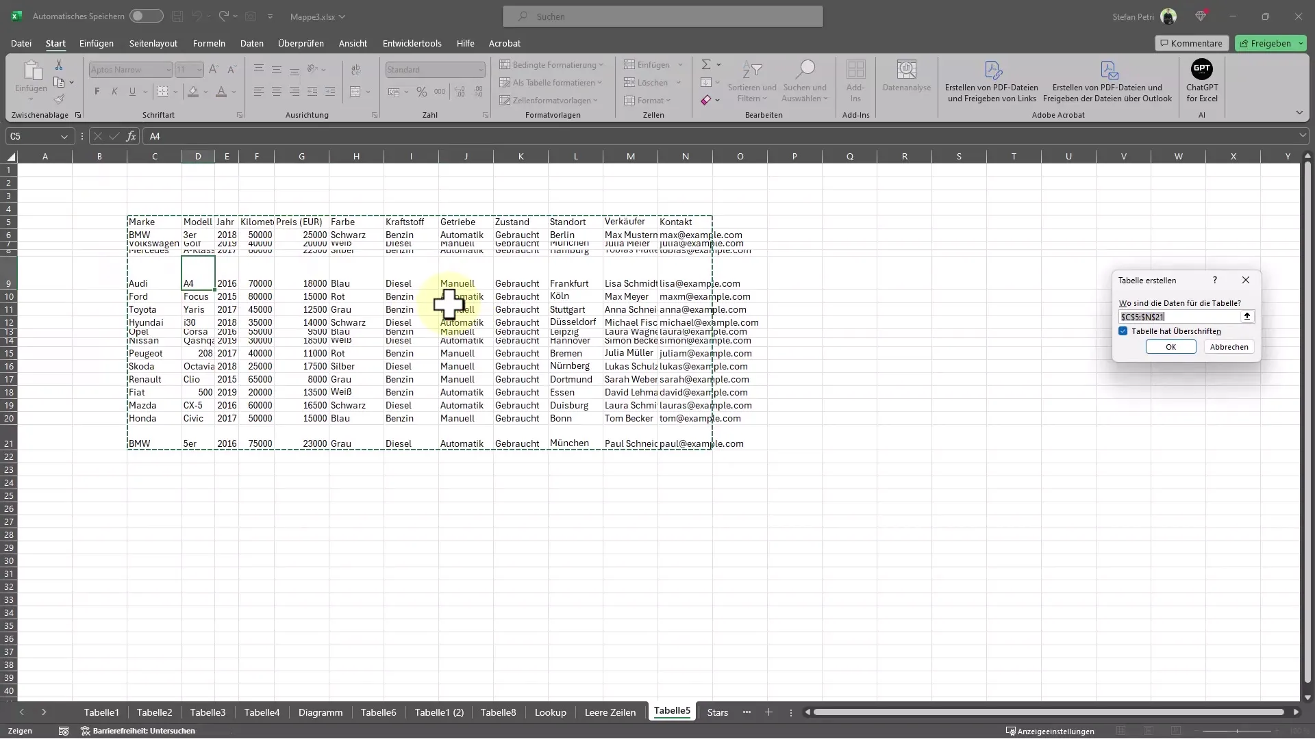
Step 3: Automatically Adjusting Row and Column Heights

To ensure your table looks neat, adjust the row and column heights. When you drag the already selected cells downwards, their height will be automatically adjusted. Note that when selecting only one cell, the adjustment is limited to that cell.

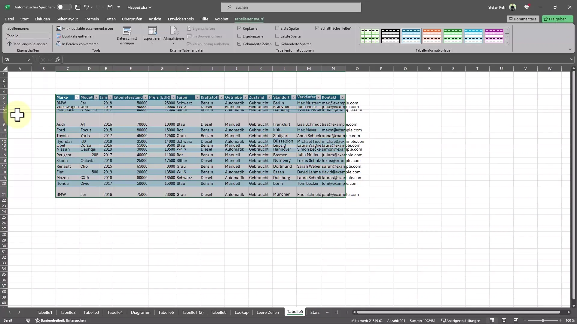
Step 4: Adjusting Column Width

If you want to adjust the column width, you can select all columns and manually drag the width. A simpler method is to use the "Ctrl + A" keyboard shortcut. Then double-click between the column headers and the widths will be automatically adjusted.

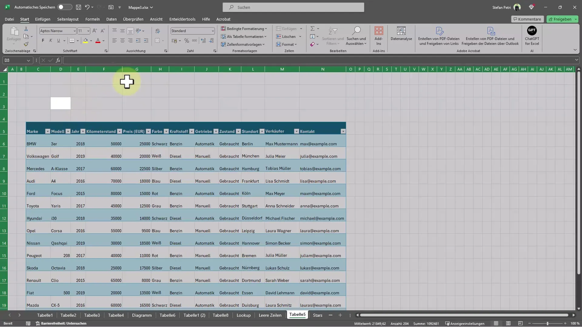
Step 5: Manually Adjusting Row Height

Sometimes, it is necessary to manually adjust the row height to create more space between the texts. Click on the row line and drag it as needed. Ideally, you want to find a balance between aesthetic design and readability.

Step 6: Centering Cells

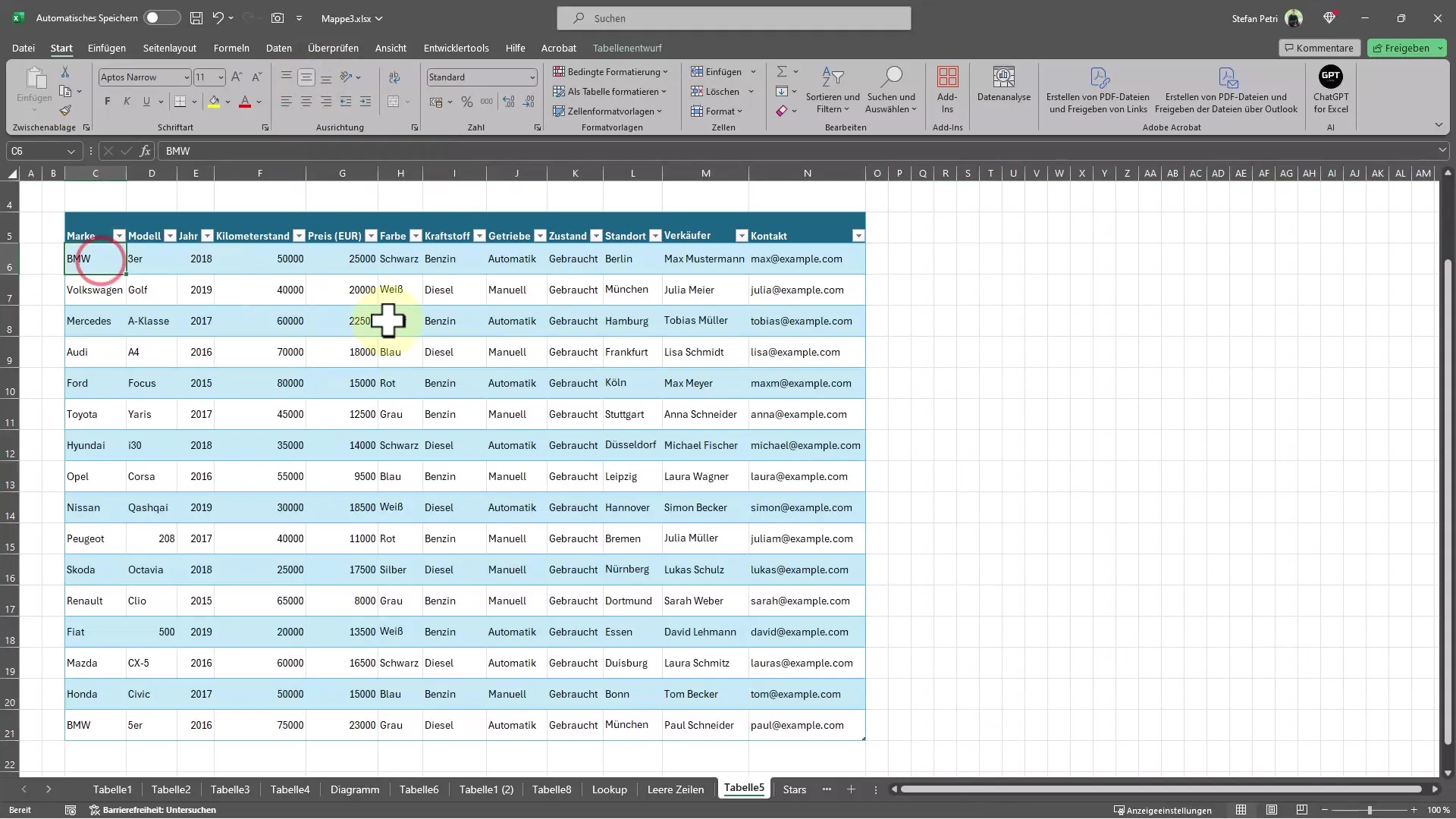
To make the text in the cells look better, align the contents centered. To do this, select the cells you want to center and click on the alignment symbol in the menu bar.

Step 7: Moving Columns

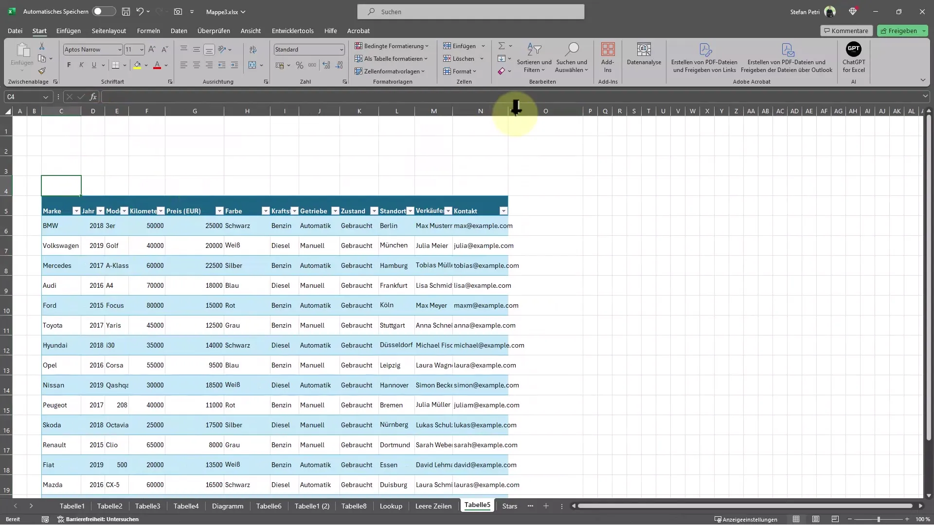
If you want to move a column, you can do so by moving the mouse to the column boundary line. Hold down the "Shift" key while adjusting the size. This will adjust the column directly across from the original without losing other content.

Step 8: Removing or Changing Filters

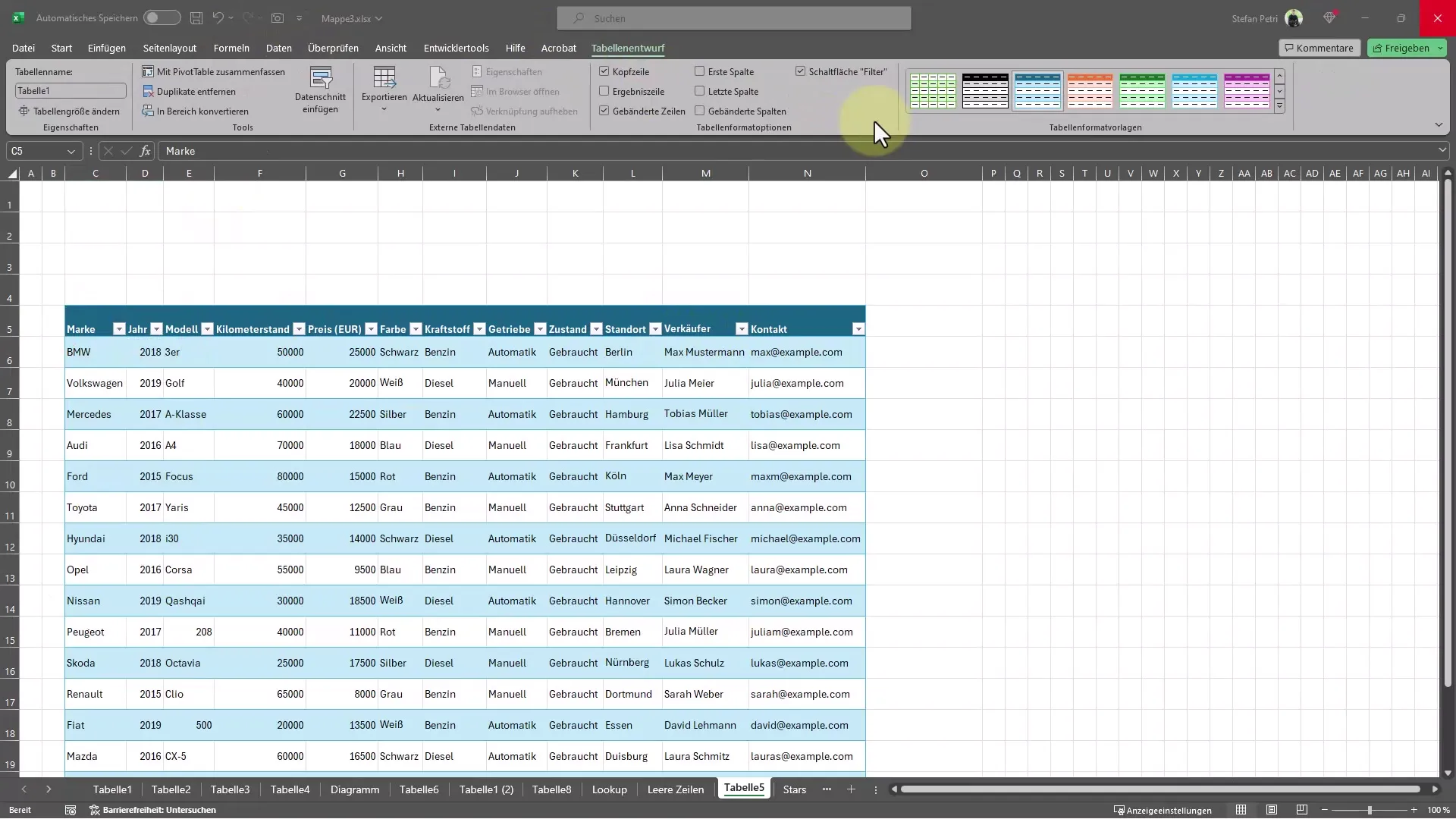
If you do not want filters in your table, go to the "Table Design" tab and deactivate the "Filter" button. Alternatively, you can also change the table's design from the respective selection and thus maintain the filter while adjusting the appearance.

Step 9: Using Templates and Designs

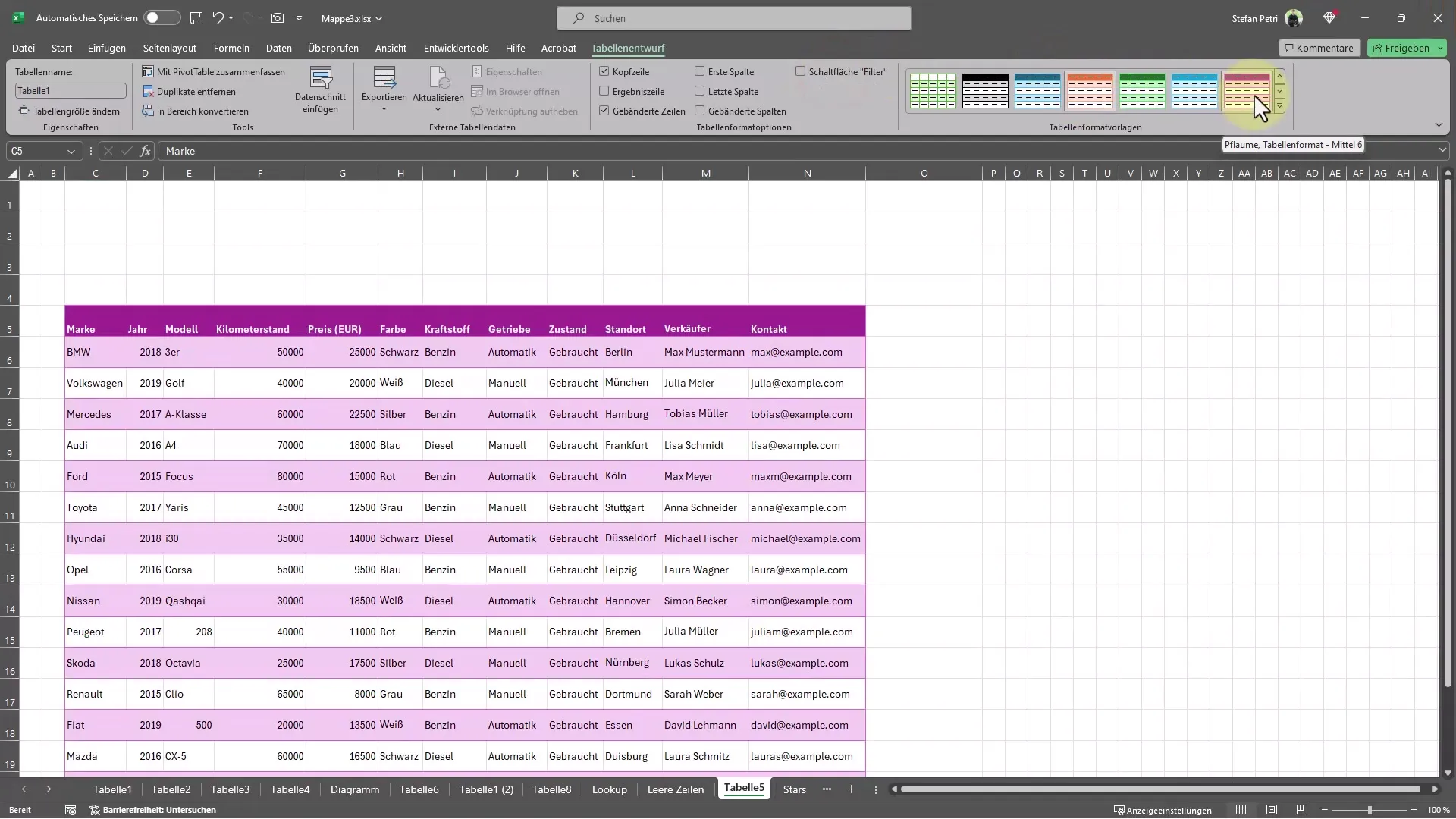
Excel offers a variety of templates and designs that are immediately applicable. You can use these to give your table a fresh, modern look. Search for various options in the "Table Design" tab and choose the style that best suits your table.

Summary

In this tutorial, you have learned how to quickly format your Excel tables. From selecting the table to adjusting column widths and using templates, you have learned all the necessary steps to make your tables look professional and appealing. Use these tips to save time and optimize your presentations.