Calculate rank and placement easily in Excel

In this short tutorial, I will show you a practical Excel function that allows you to quickly determine which rank or placement an employee or student has taken in a table. Instead of calculating the placement manually, you use a simple formula to achieve this automatically. This method is not only efficient but also particularly useful when the values in your table change. Let's get started right away!

Key Insights

The method presented uses a combination of the rank function and an absolute reference to dynamically display the placement. This way, you get the result immediately without having to take additional steps. The function updates automatically when input values change.

Step-by-Step Guide

Let's start by calculating the rank of a specific position in your table.

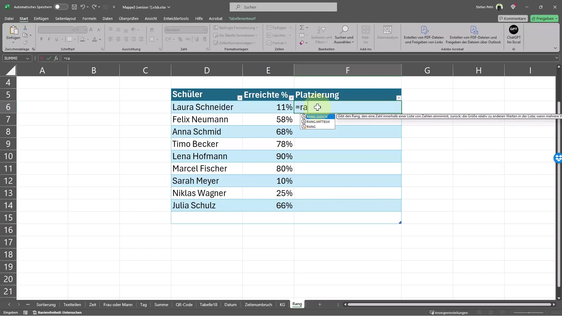
To determine a student's ranking position, you first need to navigate to the relevant cell where you want to display the result. Simply click on the cell you have chosen for this purpose.

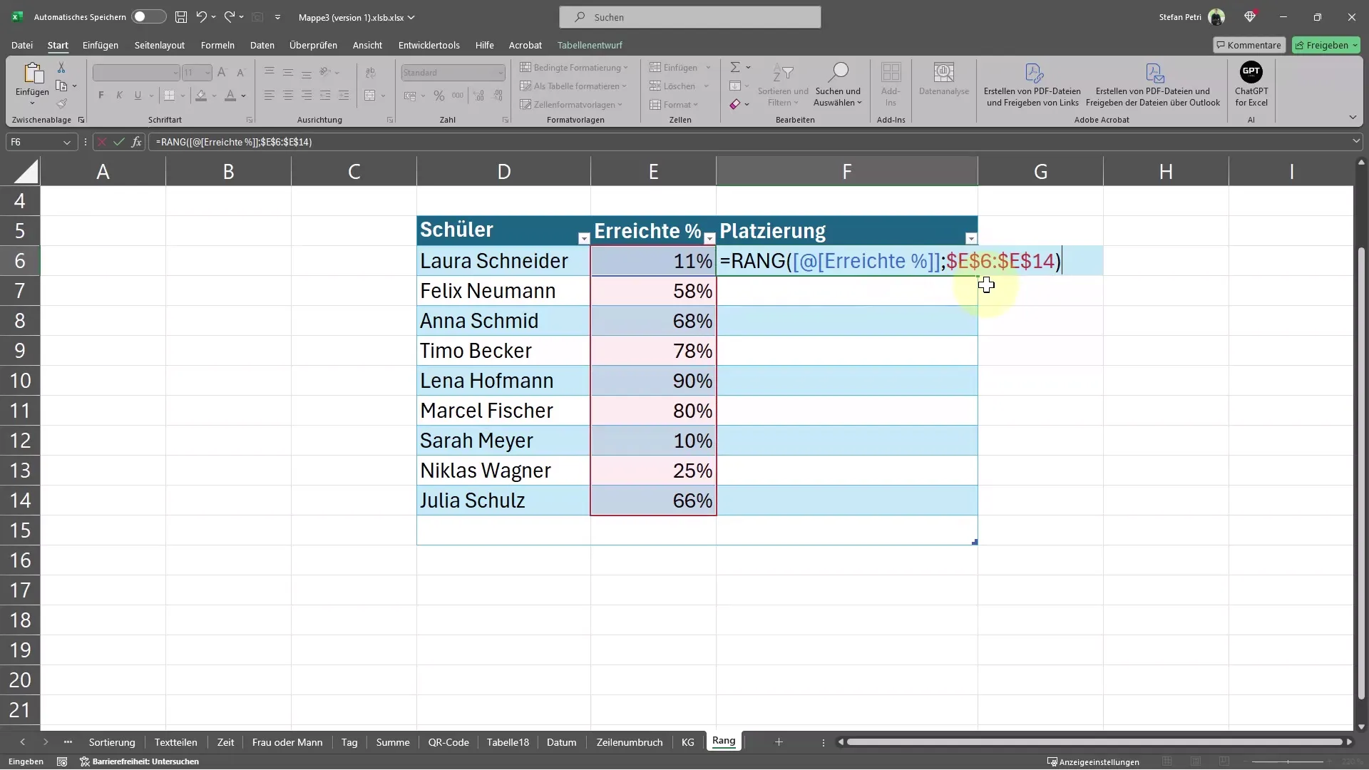
Now, you will use the rank function. This means that you must enter the formula =RANK() into the selected cell. This is the starting point for the calculation. The rank function takes two essential arguments: the value whose rank is to be determined and the reference to the entire list in which this value is compared.

Specify the reference to the entire row where the results of your students or employees are listed. It is important to ensure that the reference remains unchanged when using the formula in other cells or copying it.

To achieve this, use the F4 key. This key allows you to transform the reference to the entire list into an absolute reference. After pressing the F4 key, the reference in the formula will be correctly formatted so that it does not change in further calculations. Don't forget to close the parenthesis!

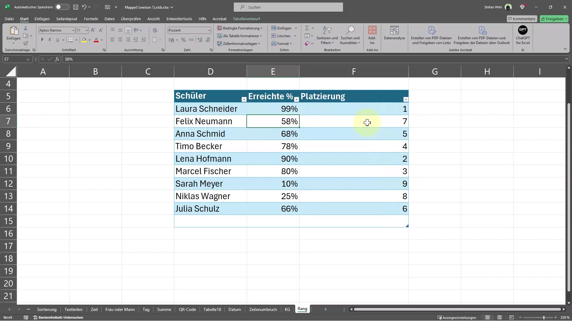
Now, you should enter a value for the rank to see how it compares to others. For example, you could enter 99% instead of the score to see what placement the student has achieved.

Upon completing the input, you will see that the placement is automatically updated. This dynamic adjustment is a particularly cool feature of Excel and immediately shows you the changed ranking order when you modify the input value.

Summary

In this guide, you have learned how to quickly and automatically determine the placement of a student or employee in Excel using the rank function. You understand the importance of setting the reference correctly to avoid calculation errors. Take advantage of this opportunity to efficiently analyze your data and save time.