Filtering data in Excel: Tips and tricks for efficiency

Filtering data in Excel is one of the fundamental functions that can greatly help you efficiently organize and analyze your data. In this guide, you will learn how to filter data easily with two different approaches. Whether you are an Excel beginner or an experienced user, these techniques will significantly simplify handling your tables.

Main Takeaways

• Filtering data in Excel can be done with just a few clicks.
• There are several approaches to apply filters to a table.
• You can easily activate and deactivate filters to display different data sets.

Step-by-Step Guide

To filter data in Excel, follow these steps:

First, open your Excel table. If you already have a table with set headers, that's ideal. To activate the filter option, you can use the shortcut Ctrl + T to format the table and add the filter option.

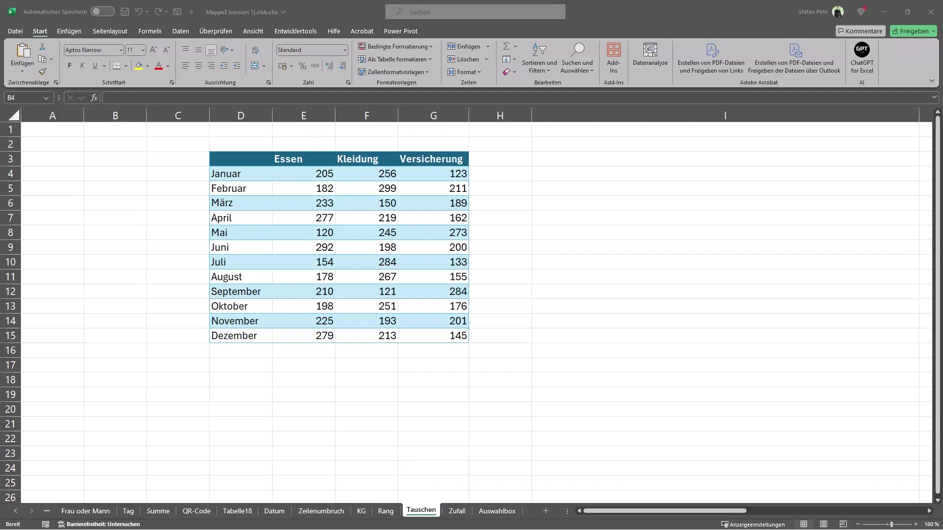
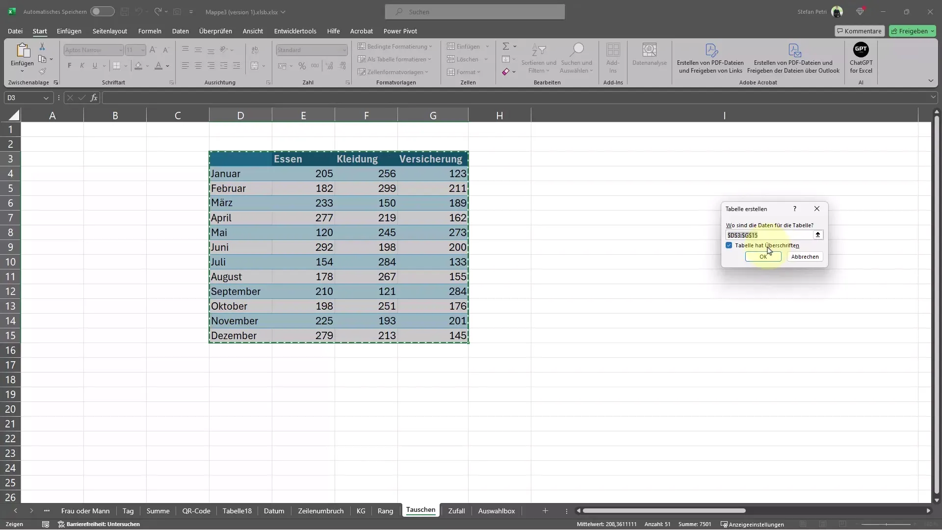
Once you have pressed Ctrl + T, you will see this window where you can easily confirm it (the checkbox should be checked for "Table has headers"):

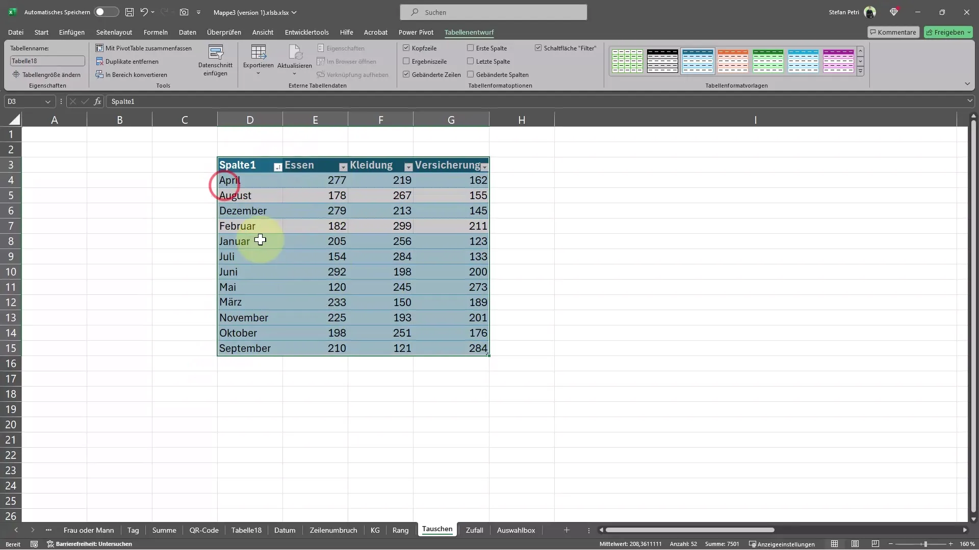
After creating the table, you have the filter options available immediately. This is done by placing filter buttons in your column headers. Now you can, for example, display filtered costs for food to see only the relevant data.

Another example could be if you wanted to sort the months in alphabetical order. This is also possible but may be less meaningful in some cases. You can reset this sorting at any time.

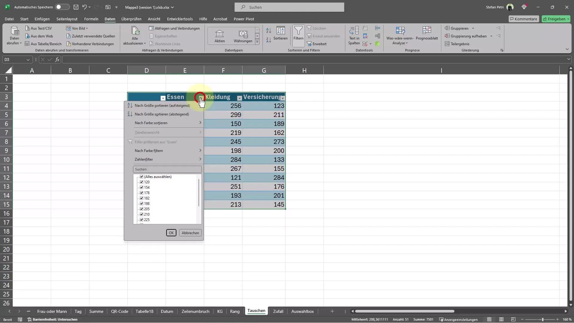
If you want to apply the filtering in a different way, you can also manually add filters. Simply select the entire table and then go to the menu and choose the Data tab and select the Filter option. This will also create a filter in your table.

With the filter activated, you can now add specific filter criteria. For example, would you like to see only expenses greater than 200 euros? This is easily possible. Choose the corresponding column and select the number filter to display only the relevant amounts.

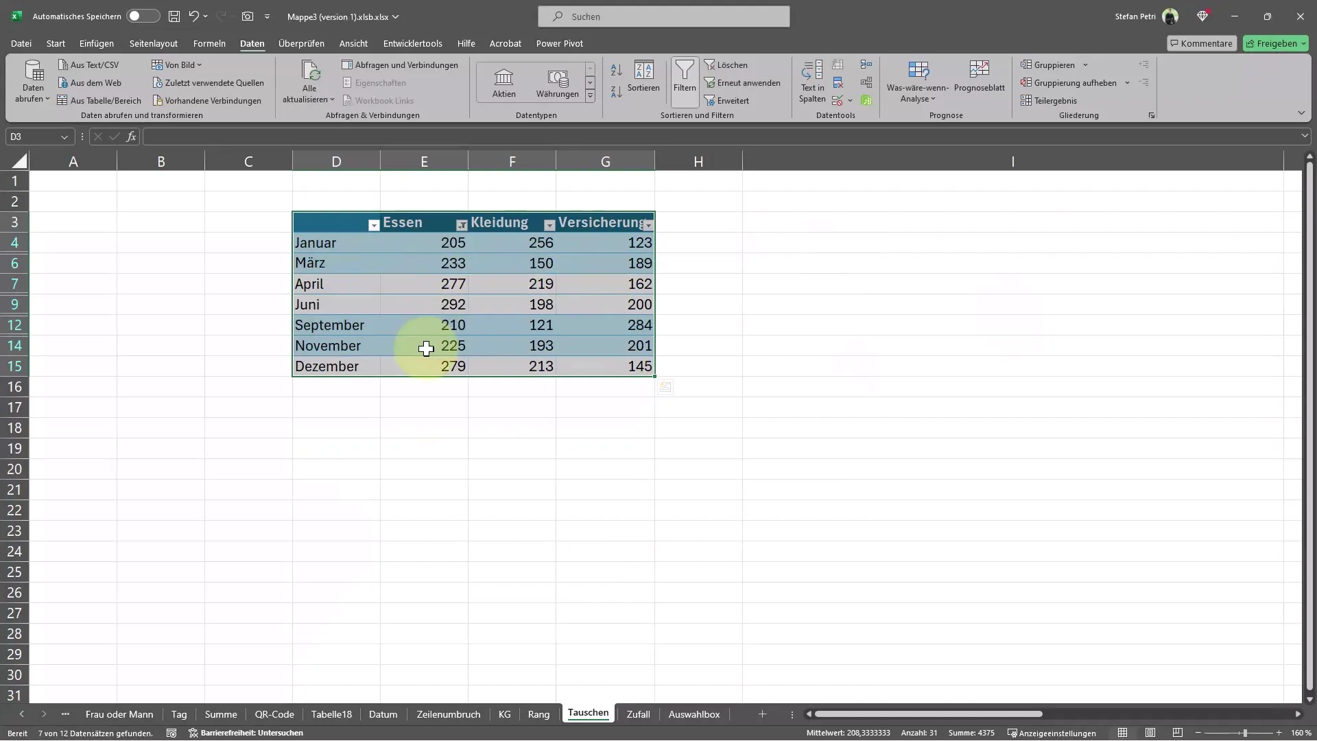
If you no longer need the filter, you can easily deactivate it. To do this, click on the filter icon and select the option Remove Filter. This will lift the filter, displaying all the data in your table. Additionally, you can access the filter options at any time by clicking back into the menu. With just one more click, you can also try out other filter applications or re-enable the filters to change the view of your data.

Summary

Filtering data in Excel is a simple yet extremely effective way to organize and analyze your data. With the steps outlined above, you can make use of both manual filters and the time-saving benefits of using shortcuts.